Getting started with lidarMiner
Hervé Guillon
27 August 2020
lidarMiner.RmdMining metadata from Rocky FTP
Most of the elevation data for the United States are hosted by the USGS on the Rocky FTP. Here, each project (and sometimes work packages within a project) is hosted in its own folder with three subfolders:
-
TIFFwhich contains the actual tiles of the dataset as large.tiffiles; -
browsewhich contains.jpgpreviews for internet browsing platforms like The National Map; -
metadatawhich contains metadata for each tile as light-weight.xmlfiles.
These metadata files can be mined with the following commands, here for California, as indicated by CA:
- Calling
mkdir dataat the root of the repository will create the/datafolder -
cd datawill change todata/ -
lftp rockyftp.cr.usgs.gov:/vdelivery/Datasets/Staged/Elevation/1m/Projectsconnects to Rocky FTP -
mirror --no-empty-dirs -n . . -i "(_CA_).*(xml)$"downloads the files matching the regular expression"(_CA_).*(xml)$".- You can kill this command once it has run past the state of interest.
- It takes around 20 min to download all the metadata for California.
Setup
For the rest of this example, we will use the packages: lidarMiner and raster (which loads sp).
Executing lidarMiner functions
This chunk executes all functions from lidarMiner, listing the files at a specified path, reading the .xml files and extracting the spatial information into a SpatialPolygonsDataFrame. The files required files are included with the package and stored in /inst/extdata that we access with system.file.
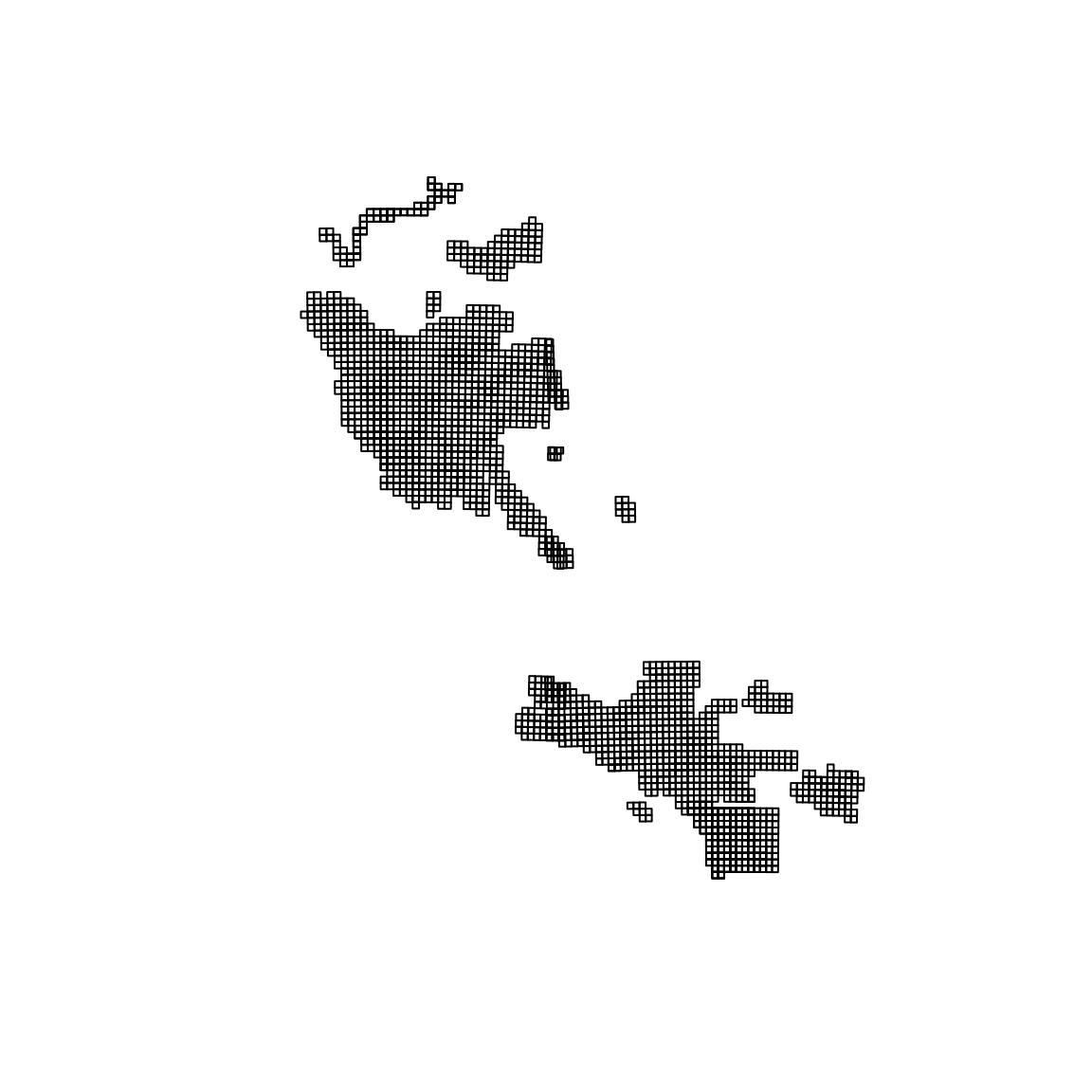
list_files <- list_lidar_files(system.file("extdata", package = "lidarMiner"))
lidar_df <- get_lidar_df(list_files)
lidar_bbox <- get_lidar_bbox(lidar_df)
plot(lidar_bbox)
Leveraging the bounding box of the lidar datasets to select the target tiles
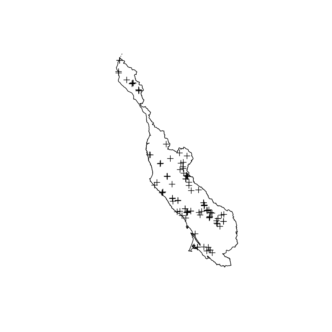
First, let’s load a region_boundary shapefile and a sampling_locations shapefile. The first describes the boundary of an area of interest, here the North Central Coast of California, USA. The second holds the locations of points of interest within the region, here field location of channel morphology sampling.
region_boundary <- shapefile(system.file("extdata", "region_boundary.shp", package = "lidarMiner"))
sampling_locations <- shapefile(system.file("extdata", "sampling_locations.shp", package = "lidarMiner"))
plot(region_boundary)
plot(sampling_locations, add = TRUE)
It might be useful to add some buffering around the point if you know how you will use the lidar datasets. For example, as I know that I will search for topographical information in squared tile \(500\times500\)-m, I add a circular buffer of \(\sqrt{2}\cdot 250\)-m around each location. This ensures that I capture enough lidar data to proceed with my downstream analysis.
Because the sampling_locations and region_boundary do not share the same CRS as lidar_bbox, this chunk handles some CRS conversions with spTransform.
region_boundary <- spTransform(region_boundary, crs(lidar_bbox))
sampling_locations <- spTransform(sampling_locations, crs(lidar_bbox))
sampling_locations_polygons <- spTransform(sampling_locations_polygons, crs(lidar_bbox))
We are now ready to perform a spatial intersect. We perform a spatial intersect with the region boundary to speed up the subsequent intersect with the sample locations.
lidar_bbox <- intersect(lidar_bbox, region_boundary)
#> Loading required namespace: rgeos
lidar_sampling_locations <- intersect(lidar_bbox, sampling_locations_polygons)
unique_networkr <- as.character(unique(lidar_sampling_locations$networkr))
plot(lidar_bbox)
plot(lidar_bbox[lidar_bbox$networkr %in% unique_networkr, ], col = "green", add = TRUE)
plot(sampling_locations_polygons, add = TRUE)
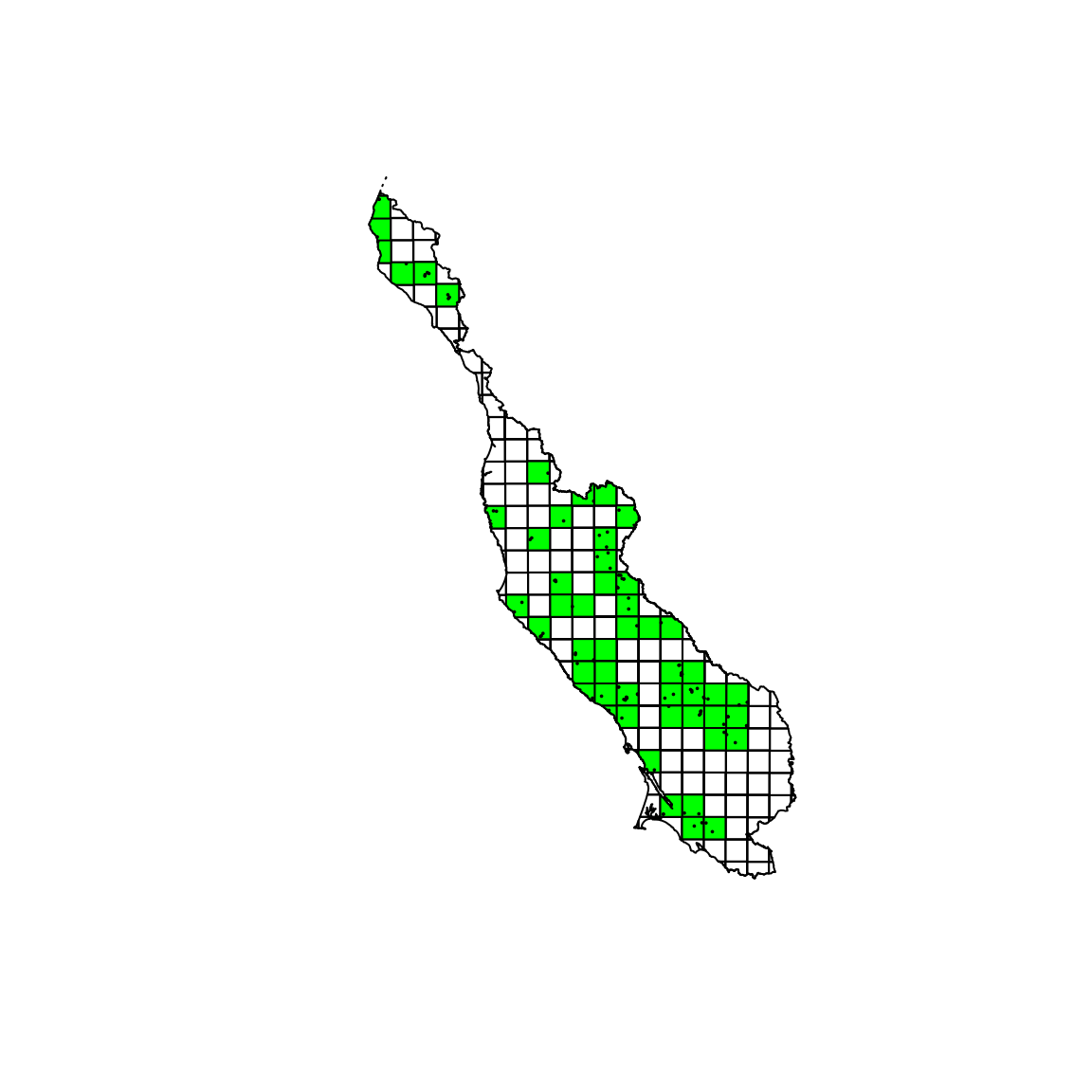
You can note that in the center of the region, two tiles have been selected thanks to the buffering.
Finally, the networkr field of the resulting lidar_sampling_locations holds the URLs of the tiles we need.
head(unique_networkr)
#> [1] "ftp://rockyftp.cr.usgs.gov/vdelivery/Datasets/Staged/Elevation/1m/Projects/CA_FEMA_R9_Mendocino_HF_2017/TIFF/USGS_one_meter_x43y435_CA_FEMA_R9_Mendocino_HF_2017.tif"
#> [2] "ftp://rockyftp.cr.usgs.gov/vdelivery/Datasets/Staged/Elevation/1m/Projects/CA_FEMA_R9_Mendocino_HF_2017/TIFF/USGS_one_meter_x44y431_CA_FEMA_R9_Mendocino_HF_2017.tif"
#> [3] "ftp://rockyftp.cr.usgs.gov/vdelivery/Datasets/Staged/Elevation/1m/Projects/CA_FEMA_R9_Mendocino_HF_2017/TIFF/USGS_one_meter_x45y430_CA_FEMA_R9_Mendocino_HF_2017.tif"
#> [4] "ftp://rockyftp.cr.usgs.gov/vdelivery/Datasets/Staged/Elevation/1m/Projects/CA_FEMA_R9_Mendocino_HF_2017/TIFF/USGS_one_meter_x45y434_CA_FEMA_R9_Mendocino_HF_2017.tif"
#> [5] "ftp://rockyftp.cr.usgs.gov/vdelivery/Datasets/Staged/Elevation/1m/Projects/CA_FEMA_R9_Mendocino_HF_2017/TIFF/USGS_one_meter_x45y437_CA_FEMA_R9_Mendocino_HF_2017.tif"
#> [6] "ftp://rockyftp.cr.usgs.gov/vdelivery/Datasets/Staged/Elevation/1m/Projects/CA_FEMA_R9_Mendocino_HF_2017/TIFF/USGS_one_meter_x46y431_CA_FEMA_R9_Mendocino_HF_2017.tif"
We can use the curl package to download all the files.
for (url in unique_networkr) curl::curl_download(url, file.path("/media/hguillon/UCD eFlow BigData1/", basename(url)))Finally, the function merge_lidar_rasters(), takes care of creating the mosaic of all the lidar files in a given folder.