Purpose

The code of fft2d(), bin() and Hann2D() is for the most part a port from Matlab to R of the code from 2DSpecTools: A 2D spectral analysis toolkit for Matlab by J. Taylor Perron et al. In consequence, a great introduction to this code is reading Perron, Kirchner, and Dietrich (2008) paper in which the authors apply spectral analysis to two examples in California (USA).

Loading data

First, we load a raster corresponding to one of the two examples from Perron, Kirchner, and Dietrich (2008), the one located near Gabilan Mesa in California.

library("statisticalRoughness")
library("rayshader")
library("raster")
gabilan_mesa <- raster(file.path(system.file("extdata/rasters/", package = "statisticalRoughness"), "gabilan_mesa.tif"))

Detrending

First, we detrend the DEM using detrend_dem() and convert it to a matrix.

summary(gabilan_mesa)
#>         gabilan_mesa
#> Min.        215.8804
#> 1st Qu.     290.5542
#> Median      311.2366
#> 3rd Qu.     331.4969
#> Max.        381.4826
#> NA's          0.0000
gabilan_mesa <- gabilan_mesa %>% detrend_dem() 
summary(gabilan_mesa)
#>         gabilan_mesa
#> Min.      -82.600540
#> 1st Qu.   -18.781493
#> Median      2.099804
#> 3rd Qu.    20.267014
#> Max.       59.039808
#> NA's        0.000000

Hillshade visualization

Here is what the area looks like. We can clearly see the imprint of Perron, Kirchner, and Dietrich (2008)’s Fig. 3a.

gabilan_mesa %>%
    raster_to_matrix() %>%
    sphere_shade(texture = "desert") %>%
    add_shadow(ray_shade(gabilan_mesa %>% raster_to_matrix(), sunaltitude = 45), max_darken = 0.3) %>%  
    add_shadow(ambient_shade(gabilan_mesa %>% raster_to_matrix()), 0) %>%
    plot_map()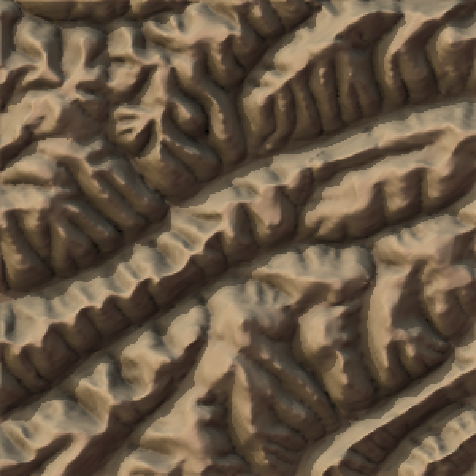

2D Fourier transform

As gabilan_mesa is already a matrix that we can pass directly to fft2d() with a Hann window (Hann = TRUE ensures that Hann2d() is called). We also bin the power spectrum using bin() and visualize the results with spectrum_plot(). For convenience, we report as a vertical line the rolloff frequency identified in Perron, Kirchner, and Dietrich (2008)’s Fig. 4a.

raster_resolution <- 9.015
FT2D <- fft2D(raster::as.matrix(gabilan_mesa), dx = raster_resolution, dy = raster_resolution, Hann = TRUE)
view_matrix(log10(Re(FT2D$spectral_power_matrix)), ply = FALSE)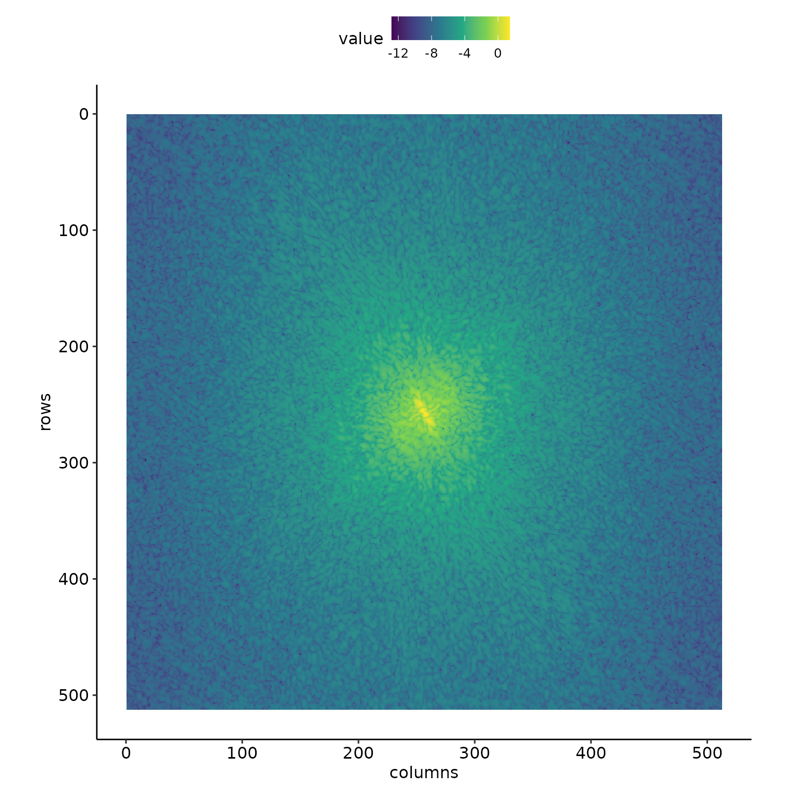

Radial power spectrum

While produced with different underlying data, this plot passes the sanity check against Perron, Kirchner, and Dietrich (2008)’s example. We can assess the break point and sloeps with get_beta(). In the graph below, the solid line corresponds to 180 m as in Perron, Kirchner, and Dietrich (2008) while the dashed-line is the change point of a segmented regression on the binned power spectrum.

nbin <- 20
binned_power_spectrum <- bin(log10(FT2D$radial_frequency_vector), log10(FT2D$spectral_power_vector), nbin)
binned_power_spectrum <- na.omit(binned_power_spectrum)
beta <- get_beta(binned_power_spectrum, FT2D)
beta
#>            fc     beta1     beta2   beta.r2
#> x 0.003577712 -2.132128 -5.431478 0.9956601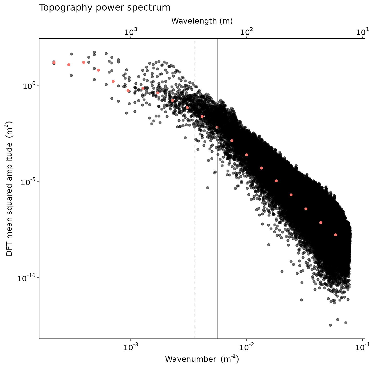

References

Perron, J. Taylor, James W. Kirchner, and William E. Dietrich. 2008. “Spectral Signatures of Characteristic Spatial Scales and Nonfractal Structure in Landscapes.” Journal of Geophysical Research: Earth Surface 113 (F4): n/a–n/a. https://doi.org/10.1029/2007JF000866.

A basic 2D Fourier analysis of topography

Hervé Guillon

08 March 2021