Example of anisotropic landscapes
Hervé Guillon
08 March 2021
zeta_examples.RmdPurpose
This vignette displays the calculation of anisotropy exponent for different landscapes: Gabilan Mesa, Yosemite Valley and Modoc Plateau.
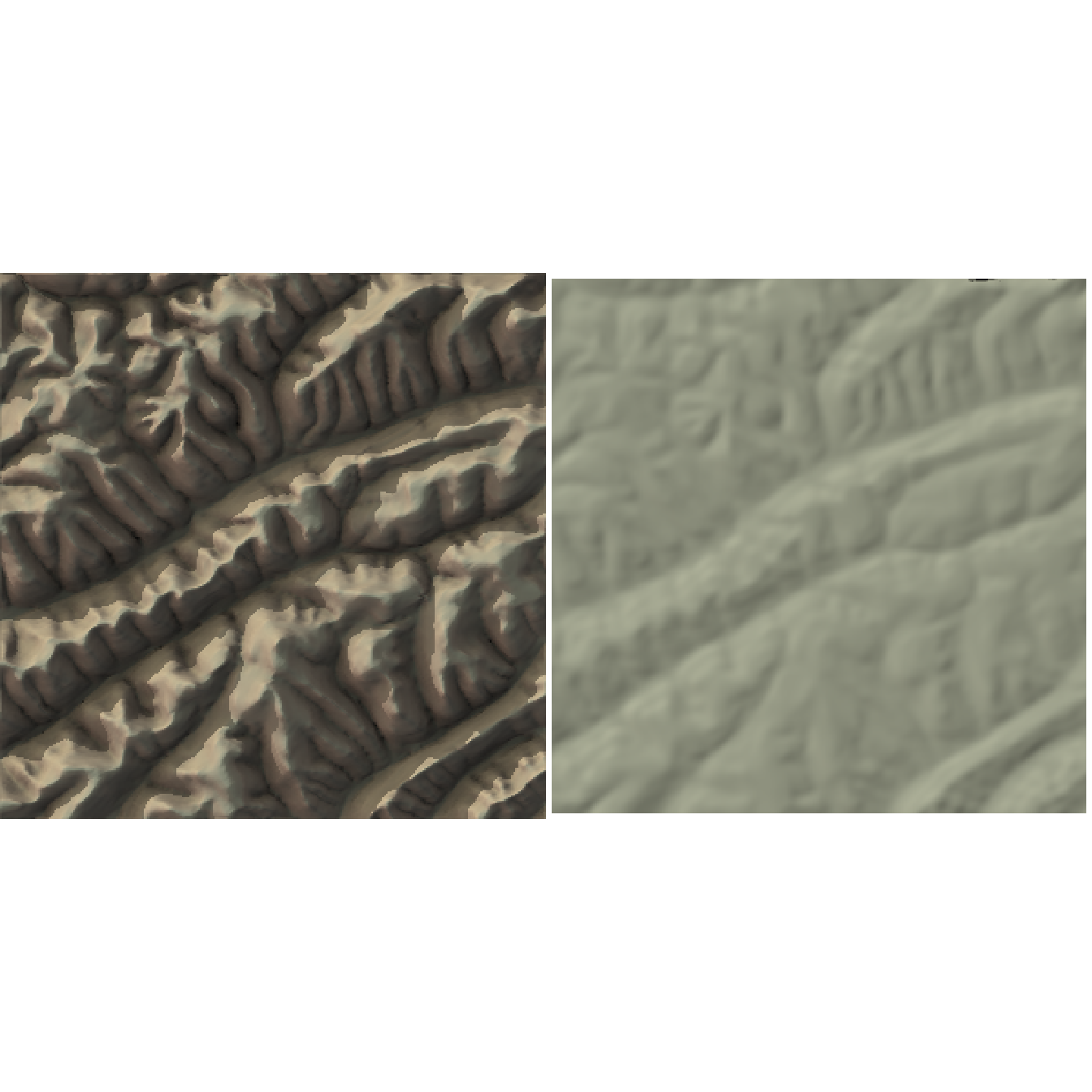
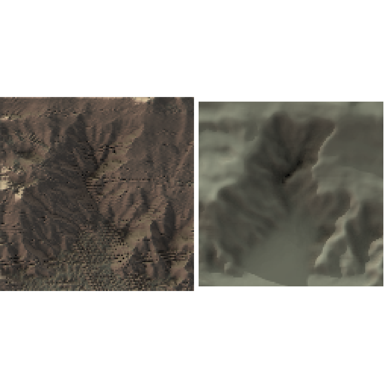
Gabilan Mesa
Gabilan Mesa landscape is the same landscape that we used in other vignettes and the test bed of Perron, Kirchner, and Dietrich (2008) methods. Using get_zeta() returns a data.frame with the variable of interest for the analysis of topographic roughness and anisotropy.
raster_resolution <- 10
gabilan_mesa <- raster::raster(file.path(system.file("extdata/rasters/", package = "statisticalRoughness"), "gabilan_mesa.tif"))
res_gabi <- get_zeta(gabilan_mesa, raster_resolution) %>% dplyr::mutate_all(signifNA)
Gabilan Mesa landscape has a minimum elevation of 215.8804016 m, an average elevation of 309.5151503 m, and a maximum elevation of 381.4825745 m. The maximum relief is thus 165.6021729 m.
The figure below showcases the landscape in its original form. The landscape was rotated so that in this original frame of reference, \(\theta_x =\) 122\(^\circ\) and \(\theta_y =\) 212\(^\circ\). (In the rotated frame of reference, \(\theta_x' = 0^\circ\) and \(\theta_y' = 90^\circ\).) The segmented regression on the power spectrum identifies scalings with slope \(\beta_1 =\) -2.13, and \(\beta_2 =\) -5.43, before and after a cut-off lengthscale of \(1/f_c =\) 310 m, respectively. As \(\beta = 2H + d\), and \(d = 2\), the Hurst coefficients \(H\) corresponding to \(\beta_1\) and \(\beta_2\) are 0.065, and 1.715, respectively. Before a cut-off lengthscale of 127 m, the roughness exponents in the \(x\)– and \(y\)–directions are \(\alpha_{1,x} =\) 0.764, and \(\alpha_{1,y} =\) 0.668. Consequently, the anisotropy exponent is \(\zeta_1 =\) 1.14. After cut-off lengthscale, the roughness exponents are lower and almost equal with \(\alpha_{2,x} =\) 0.302, and \(\alpha_{2,y} =\) 0.259. Consequently, the anisotropy exponent is \(\zeta_2 =\) 1.17.
The figure below showcases the landscape in its original form (left) and smoothed with a Gaussian kernel of 12 standard deviations to match the value of \(r_c\) (right).
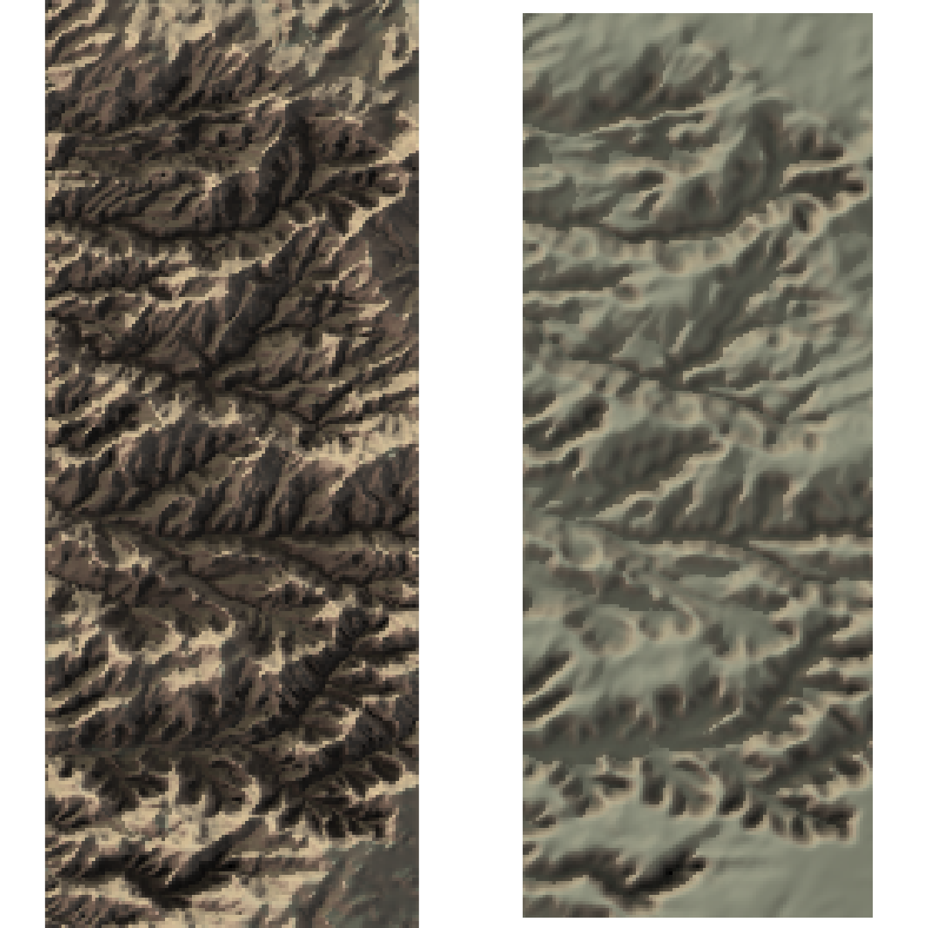
Yosemite Valley
raster_resolution <- 10
yosemite <- raster::raster(file.path(system.file("extdata/rasters/", package = "statisticalRoughness"), "yosemite.tif"))
res_yose <- get_zeta(yosemite, raster_resolution) %>% dplyr::mutate_all(signifNA)
Yosemite Valley landscape has a minimum elevation of 1217.6658936 m, an average elevation of 1710.8465941 m, and a maximum elevation of 2696.1628418 m. The maximum relief is thus 1478.4969482 m. The figure below showcases the landscape in its original form. The landscape was rotated so that in this original frame of reference, \(\theta_x =\) 122\(^\circ\) and \(\theta_y =\) 212\(^\circ\). (In the rotated frame of reference, \(\theta_x' = 0^\circ\) and \(\theta_y' = 90^\circ\).) The segmented regression on the power spectrum identifies scalings with slope \(\beta_1 =\) -4.94, and \(\beta_2 =\) -4.23, before and after a cut-off lengthscale of \(1/f_c =\) 485 m, respectively. As \(\beta = 2H + d\), and \(d = 2\), the Hurst coefficients \(H\) corresponding to \(\beta_1\) and \(\beta_2\) are 1.47, and 1.115. Before a cut-off lengthscale of 290 m, the roughness exponents in the \(x\)– and \(y\)–directions are \(\alpha_{1,x} =\) 0.568, and \(\alpha_{1,y} =\) 0.588. Consequently, the anisotropy exponent is \(\zeta_1 =\) 0.966. After cut-off lengthscale, the roughness exponents are lower and almost equal with \(\alpha_{2,x} =\) 0.36, and \(\alpha_{2,y} =\) 0.306. Consequently, the anisotropy exponent is \(\zeta_2 =\) 1.18.
The figure below showcases the landscape in its original form (left) and smoothed with a Gaussian kernel of 29 standard deviations to match the value of \(r_c\) (right).
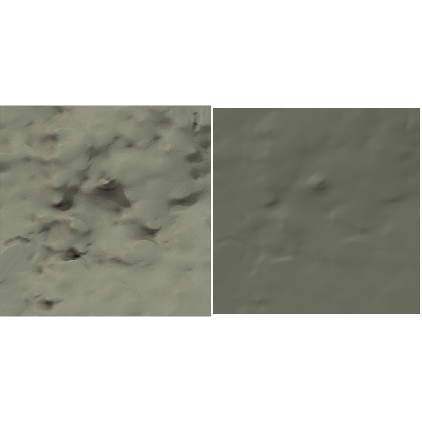
Modoc Plateau
raster_resolution <- 10
modoc <- raster::raster(file.path(system.file("extdata/rasters/", package = "statisticalRoughness"), "modoc.tif"))
res_modo <- get_zeta(modoc, raster_resolution) %>% dplyr::mutate_all(signifNA)
Modoc Plateau landscape has a minimum elevation of 1421.567749 m, an average elevation of 1448.5727549 m, and a maximum elevation of 1476.7843018 m. The maximum relief is thus 55.2165527 m. The landscape was rotated so that in this original frame of reference, \(\theta_x =\) 91.6\(^\circ\) and \(\theta_y =\) 181.6\(^\circ\). (In the rotated frame of reference, \(\theta_x' = 0^\circ\) and \(\theta_y' = 90^\circ\).) The segmented regression on the power spectrum identifies scalings with slope \(\beta_1 =\) -2.39, and \(\beta_2 =\) -5.22, before and after a cut-off lengthscale of \(1/f_c =\) 780 m, respectively. As \(\beta = 2H + d\), and \(d = 2\), the Hurst coefficients \(H\) corresponding to \(\beta_1\) and \(\beta_2\) are 0.195, and 1.61. Before a cut-off lengthscale of 291 m, the roughness exponents in the \(x\)– and \(y\)–directions are almost equal as \(\alpha_{1,x} =\) 0.635, and \(\alpha_{1,y} =\) 0.682. Consequently, the anisotropy exponent is \(\zeta_1 =\) 0.93. After cut-off lengthscale, the roughness exponents are more distinct as \(\alpha_{2,x} =\) 0.343, and \(\alpha_{2,y} =\) 0.34. However, the anisotropy exponent, \(\zeta_2\), cannot be derived as at least one ofthe distribution of \(\alpha_2\) has a large spread and its mean is an inconclusive description of centrality.
The figure below showcases the landscape in its original form (left) and smoothed with a Gaussian kernel of 29 standard deviations to match the value of \(r_c\) (right).
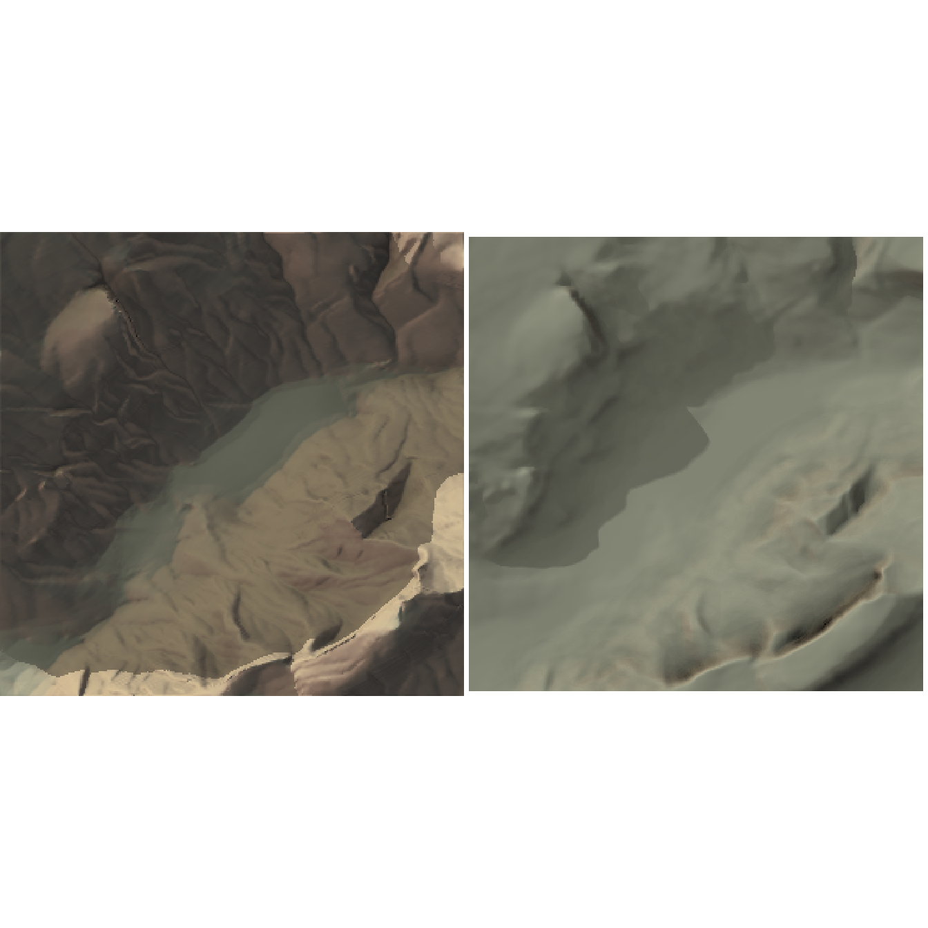
Marble Canyon
raster_resolution <- 90
marble_canyon <- raster::raster(file.path(system.file("extdata/rasters/", package = "statisticalRoughness"), "marble_canyon.tif"))
marble_canyon <- raster::aggregate(marble_canyon, fact = 9) # 90 m to match Pastor-Satorras
res_mrbl <- get_zeta(marble_canyon, raster_resolution) %>% dplyr::mutate_all(signifNA)
Marble Canyon landscape has a minimum elevation of 1545.6765544 m, an average elevation of 1862.2165704 m, and a maximum elevation of 2193.9054754 m. The maximum relief is thus 648.228921 m.
The figure below showcases the landscape in its original form. The landscape was rotated so that in this original frame of reference, \(\theta_x =\) 71.9\(^\circ\) and \(\theta_y =\) 161.9\(^\circ\). (In the rotated frame of reference, \(\theta_x' = 0^\circ\) and \(\theta_y' = 90^\circ\).) The segmented regression on the power spectrum identifies scalings with slope \(\beta_1 =\) -1.76, and \(\beta_2 =\) -3.66, before and after a cut-off lengthscale of \(1/f_c =\) 2220 m, respectively. As \(\beta = 2H + d\), and \(d = 2\), the Hurst coefficients \(H\) corresponding to \(\beta_1\) and \(\beta_2\) are -0.12, and 0.83, respectively. Before a cut-off lengthscale of 635 m, the roughness exponents in the \(x\)– and \(y\)–directions are \(\alpha_{1,x} =\) 0.578, and \(\alpha_{1,y} =\) 0.544. Consequently, the anisotropy exponent is \(\zeta_1 =\) 1.06. After cut-off lengthscale, the roughness exponents are lower and almost equal with \(\alpha_{2,x} =\) 0.243, and \(\alpha_{2,y} =\) 0.257. Consequently, the anisotropy exponent is \(\zeta_2 =\) -.
The figure below showcases the landscape in its original form (left) and smoothed with a Gaussian kernel of 7 standard deviations to match the value of \(r_c\) (right).
Submarine Canyon
raster_resolution <- 50
submarine_canyon <- raster::raster(file.path(system.file("extdata/rasters/", package = "statisticalRoughness"), "submarine_canyon.tif"))
res_subm <- get_zeta(submarine_canyon, raster_resolution) %>% dplyr::mutate_all(signifNA)
Submarine Canyon landscape has a minimum elevation of -2300.2202148 m, an average elevation of -1773.067128 m, and a maximum elevation of -957.03302 m. The maximum relief is thus 1343.1871948 m.
The figure below showcases the landscape in its original form. The landscape was rotated so that in this original frame of reference, \(\theta_x =\) 91.6\(^\circ\) and \(\theta_y =\) 181.6\(^\circ\). (In the rotated frame of reference, \(\theta_x' = 0^\circ\) and \(\theta_y' = 90^\circ\).) The segmented regression on the power spectrum identifies scalings with slope \(\beta_1 =\) -6.32, and \(\beta_2 =\) -3.2, before and after a cut-off lengthscale of \(1/f_c =\) 1200 m, respectively. As \(\beta = 2H + d\), and \(d = 2\), the Hurst coefficients \(H\) corresponding to \(\beta_1\) and \(\beta_2\) are 2.16, and 0.6, respectively. Before a cut-off lengthscale of 698 m, the roughness exponents in the \(x\)– and \(y\)–directions are \(\alpha_{1,x} =\) 0.663, and \(\alpha_{1,y} =\) 0.592. Consequently, the anisotropy exponent is \(\zeta_1 =\) 1.12. After cut-off lengthscale, the roughness exponents are lower and almost equal with \(\alpha_{2,x} =\) 0.368, and \(\alpha_{2,y} =\) 0.353. Consequently, the anisotropy exponent is \(\zeta_2 =\) 1.04.
The figure below showcases the landscape in its original form (left) and smoothed with a Gaussian kernel of 13 standard deviations to match the value of \(r_c\) (right).
Comparing Landscapes
The following table summarizes the metrics for the three landscapes.
res <- rbind(res_gabi, res_yose, res_modo, res_mrbl, res_subm) %>%
  dplyr::select(-c("w", "xi", "alpha1", "alpha2"))
rownames(res) <- c("Gabilan Mesa", "Yosemite Valley", "Modoc Plateau", "Marble Canyon", "Submarine Canyon")| \(\beta_1\) | \(\beta_2\) | \(\alpha_{1,x}\) | \(\alpha_{1,y}\) | \(\zeta_1\) | \(\alpha_{2,x}\) | \(\alpha_{2,y}\) | \(\zeta_2\) | \(\theta\) | \(1/f_c\) | \(r_c\) | \(\xi_x\) | \(\xi_y\) | \(w_x\) | \(w_y\) | |
|---|---|---|---|---|---|---|---|---|---|---|---|---|---|---|---|
| Gabilan Mesa | -2.13 | -5.43 | 0.764 | 0.668 | 1.140 | 0.302 | 0.259 | 1.17 | 302.0 | 310 | 127 | 130 | 127 | 21.80 | 12.90 |
| Yosemite Valley | -4.94 | -4.23 | 0.568 | 0.588 | 0.966 | 0.360 | 0.306 | 1.18 | 302.0 | 485 | 290 | 308 | 230 | 249.00 | 72.50 |
| Modoc Plateau | -2.39 | -5.22 | 0.635 | 0.682 | 0.930 | 0.343 | 0.340 |
|
91.6 | 780 | 291 | 323 | 258 | 4.38 | 2.74 |
| Marble Canyon | -1.76 | -3.66 | 0.578 | 0.544 | 1.060 | 0.243 | 0.257 |
|
71.9 | 2220 | 635 | 663 | 584 | 86.00 | 64.30 |
| Submarine Canyon | -6.32 | -3.20 | 0.663 | 0.592 | 1.120 | 0.368 | 0.353 | 1.04 | 91.6 | 1200 | 698 | 679 | 716 | 91.40 | 90.30 |
While the estimate of statistical roughness from \(\beta\) and \(\alpha\) values differ for the three landscapes, their interpretations are coherent.
Gabilan Mesa landscape is weakly anisotropic and mainly correlated below 127 m, and isotropic and mainly anti-correlated above 127 m. Yosemite Valley landscape is anisotropic and mainly correlated below 290 m, and isotropic with no clear correlation above 290 m. Modoc Plateau landscape is isotropic and mainly correlated below 291 m, and with undetermined behaviour above 291 m.
References
Perron, J. Taylor, James W. Kirchner, and William E. Dietrich. 2008. “Spectral Signatures of Characteristic Spatial Scales and Nonfractal Structure in Landscapes.” Journal of Geophysical Research: Earth Surface 113 (F4): n/a–n/a. https://doi.org/10.1029/2007JF000866.