Purpose

The main purpose of Fourier analysis in this package is to rotate rasters so that they face the main components of the two-dimensional Fourier spectrum.

Loading data

First, we perform the basic steps from this vignette.

library("statisticalRoughness")
library("rayshader")
library("raster")

gabilan_mesa <- raster(file.path(system.file("extdata/rasters/", package = "statisticalRoughness"), "modoc.tif"))
gabilan_mesa <- gabilan_mesa %>% detrend_dem() 
raster_resolution <- 9.015
FT2D <- fft2D(raster::as.matrix(gabilan_mesa), dx = raster_resolution, dy = raster_resolution, Hann = TRUE)
nbin <- 20
binned_power_spectrum <- bin(log10(FT2D$radial_frequency_vector), log10(FT2D$spectral_power_vector), nbin)
binned_power_spectrum <- na.omit(binned_power_spectrum)

Removing the background spectrum

Then we obtain a normalized spectral power matrix by removing the background spectrum. More details are provided in Perron, Kirchner, and Dietrich (2008).

normalized_spectral_power_matrix <- get_normalized_spectral_power_matrix(binned_power_spectrum, FT2D)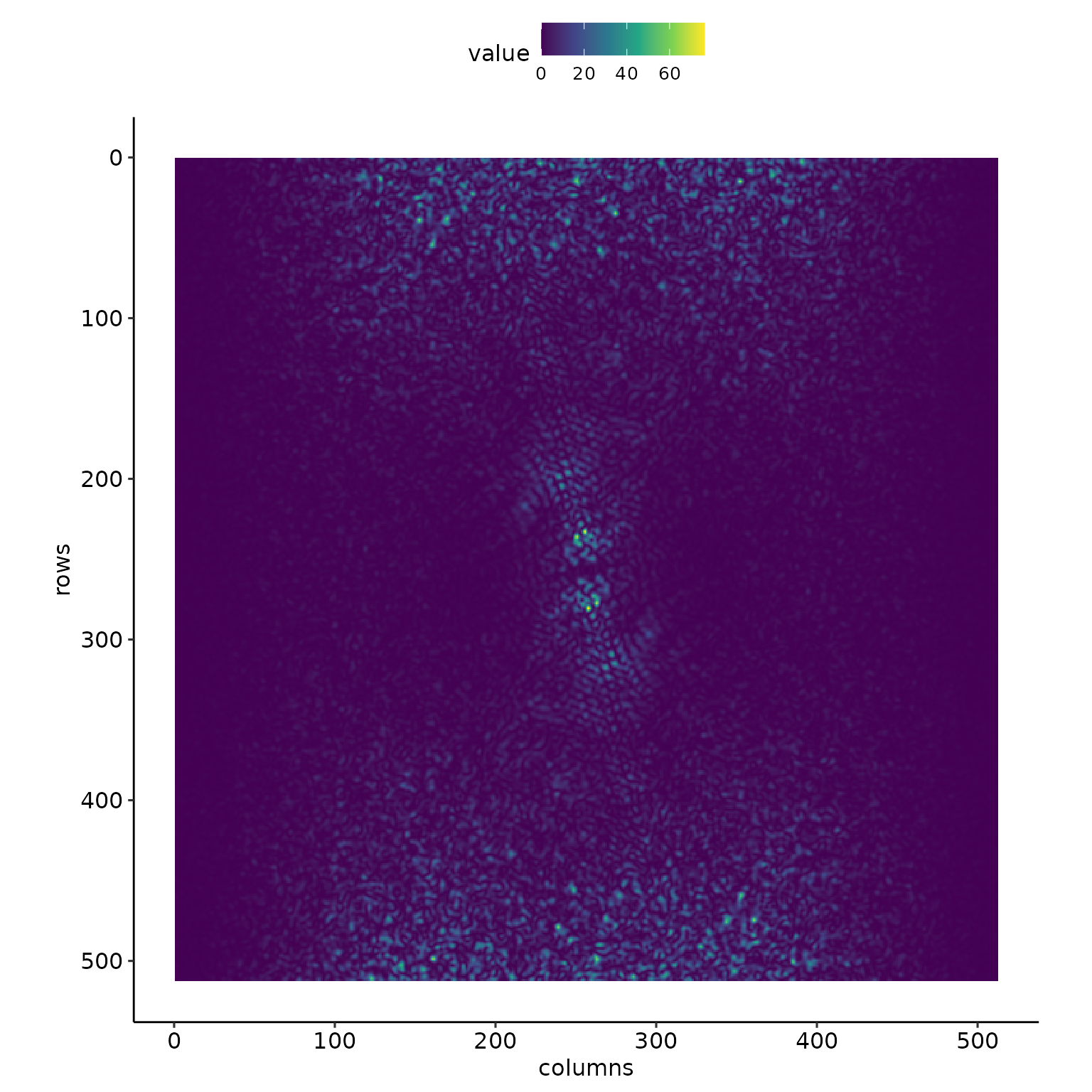

Filtering the spectral power matrix

This normalized spectral power matrix is then filtered to identify main components. While Perron, Kirchner, and Dietrich (2008) used a comparison with a \(\chi^2\) distribution, we keep the values spectral power that are above the 99.99th percentile of the logarithm of their values. The plot below corresponds, albeit not exactly, to their Fig. 3c.

filtered_spectral_power_matrix <- filter_spectral_power_matrix(normalized_spectral_power_matrix, FT2D, quantile_prob = c(0.9999))

Extracting the angle

ang_fourier <- get_fourier_angle(filtered_spectral_power_matrix, FT2D)

From the filtered spectral power matrix, get_fourier_angle() extracts the maximum value of a circular density. In the current example, that angle \(\theta\) is \(\simeq\) 92. In their paper, Perron, Kirchner, and Dietrich (2008) identifies the main direction at 131\(^\circ\) and a secondary one at 45\(^\circ\). The mod(180) we found is 92\(^\circ\), a value close to the one from Perron, Kirchner, and Dietrich (2008). As shown in the rose plot below, the secondary peak at around 45\(^\circ\) is also well captured. While the agreement is satisfactory, multiple factors explain the discrepancies between the two values:

the underlying data are slightly different: Perron, Kirchner, and Dietrich (2008) uses a 4-m raster, resampled from lidar data; we use a 10-m DEM;
the filtering of the normalized power spectrum are different;
the extent of the two regions are slightly different.

Rotating the raster

Now that we have an angle for the rotation, we use the rotate_raster() function to turn the raster along the main direction. This mean that the rows and columns of the underlying matrix are parallel or orthogonal to the main component of the 2D Fourier transform.

Original topography

Rotated topography

Notice how the main valleys are now oriented North-South because they are perpendicular to the main East-West undulations we identified.

References

Perron, J. Taylor, James W. Kirchner, and William E. Dietrich. 2008. “Spectral Signatures of Characteristic Spatial Scales and Nonfractal Structure in Landscapes.” Journal of Geophysical Research: Earth Surface 113 (F4): n/a–n/a. https://doi.org/10.1029/2007JF000866.

Rotating rasters along 2DFT main components

Hervé Guillon

08 March 2021