library(RiverML)
library(magrittr)

Merging benchmark results

The output files from the HPC are organized with one folder per learner and sub-folders for regions. The following snippet merges all the benchmark results using getAllBMRS().

PATH <- "F:/hguillon/research/regional_benchmark/"
dirs <- list.dirs(PATH, recursive = FALSE, full.names = FALSE)

bmrs <- lapply(dirs, function(dir){getAllBMRS(file.path(PATH, dir), pattern = paste0(dir, "_"))})
bmrs_perf <- lapply(bmrs, function(bmr) bmr$perf)
bmrs_tune <- lapply(bmrs[dirs != "baseline"], function(bmr) bmr$tune  %>% distinct())

BMR_res <- list()
BMR_res$perf <- do.call(rbind, bmrs_perf)
BMR_res$tune <-  bmrs_tune[[1]]
for (i in seq_along(bmrs_tune)[-1]) BMR_res$tune <- full_join(BMR_res$tune, bmrs_tune[[i]])

The associated results in BMR_res are provided with the package.

data("BMR_res")
BMR_perf <- getBMR_perf_tune(BMR_res, type = "perf")
BMR_perf %>% dplyr::sample_n(10) %>%
    knitr::kable(digits = 3, format = "html", caption = "benchmark results") %>%
    kableExtra::kable_styling(bootstrap_options = c("hover", "condensed")) %>%
    kableExtra::scroll_box(width = "7in", height = "5in")

benchmark results
task.id	learner.id	iter	multiclass.au1u	acc	mmce	multiclass.aunu	timetrain	FS_NUM
NC	randomForest	100	0.968	0.853	0.147	0.967	130.775	45
SECA	naiveBayes	15	0.950	0.667	0.333	0.871	0.040	11
SAC	naiveBayes	28	0.836	0.255	0.745	0.759	0.010	5
K	kknn	19	0.944	0.848	0.152	0.939	0.000	6
SC	nnTrain	54	0.819	0.462	0.538	0.784	1205.046	6
SJT	kknn	38	0.992	0.750	0.250	0.992	0.010	8
K	naiveBayes	18	0.904	0.656	0.344	0.905	0.010	10
NC	randomForest	21	0.939	0.794	0.206	0.941	64.493	15
SFE	featureless	50	0.500	0.095	0.905	0.500	0.030	30
SC	kknn	88	0.858	0.615	0.385	0.849	0.030	18

Processing benchmark results

Performance plots

makeAverageAUCPlot(BMR_perf) + ggplot2::scale_x_continuous(breaks = c(5, 25, 50))

makeAverageAccPlot(BMR_perf) + ggplot2::scale_x_continuous(breaks = c(5, 25, 50))

makeTotalTimetrainPlot(BMR_perf) + ggplot2::scale_x_continuous(breaks = c(5, 25, 50))

Model selection

The model selection is handled by examining statistical differences between the distribution of performance metrics for successive iterations of model training with an increasing number of predictors. On the following graph, the brackets indicate statistically significant differences between the distribution assessed by a Dunn test for the SAC region and the randomForest learner.

makeExampleModelSelectionPlot(BMR_perf, lrn = c("randomForest"), window_size = 7)[["SAC"]]

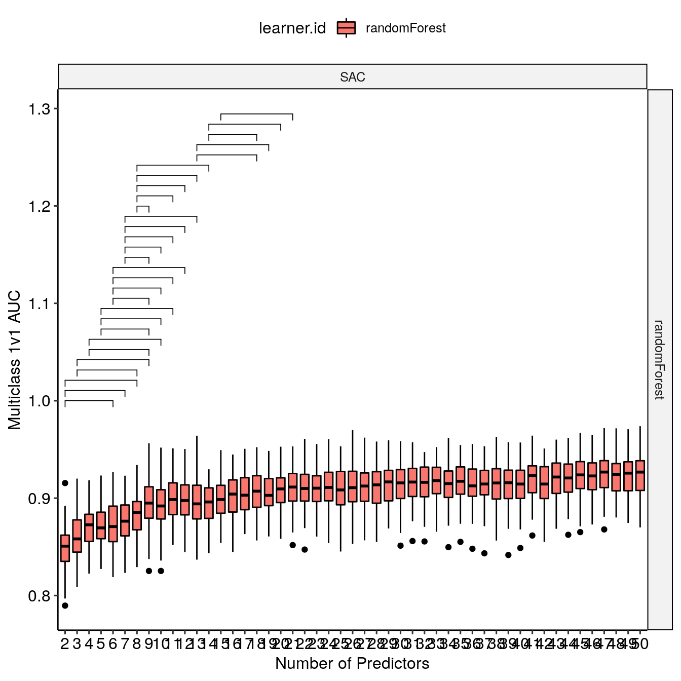
The p-value is internally ajusted to take into account multiple comparison with a Bonferroni correction. The search window influence (window_size) is examined with makeWindowInfluencePlot() which requires use to declare where we are storing the names of the selected features for each iterations.

selectedPATH <- system.file("extdata/selectedFeatures/", package = "RiverML")

makeWindowInfluencePlot(BMR_perf, selectedPATH, lrn = "randomForest") +
    ggplot2::xlim(c(0,20))

The window size selection is mainly based on the evolution of the number of optimal predictors per classes in a given region of study with respect to the window size. This balances a trade-off between two effects. A large window increases the likelihood to find a statistically different performance distribution is high and selects a large number of predictors. A small window decreases the likelihood to find statistically significant difference but might miss the inclusion of an important predictor leading to a significant increase in performance. In our example above, with a window size of 8, there is a major jump in the number of predictors per class which increases the likelihood of overfit for the optimal models.

Feature importance

The optimal feature sets are obtained for each learner by using get_bestFeatureSets().

bestFeatureSets <- get_bestFeatureSets(BMR_perf, selectedPATH, window_size = 7)

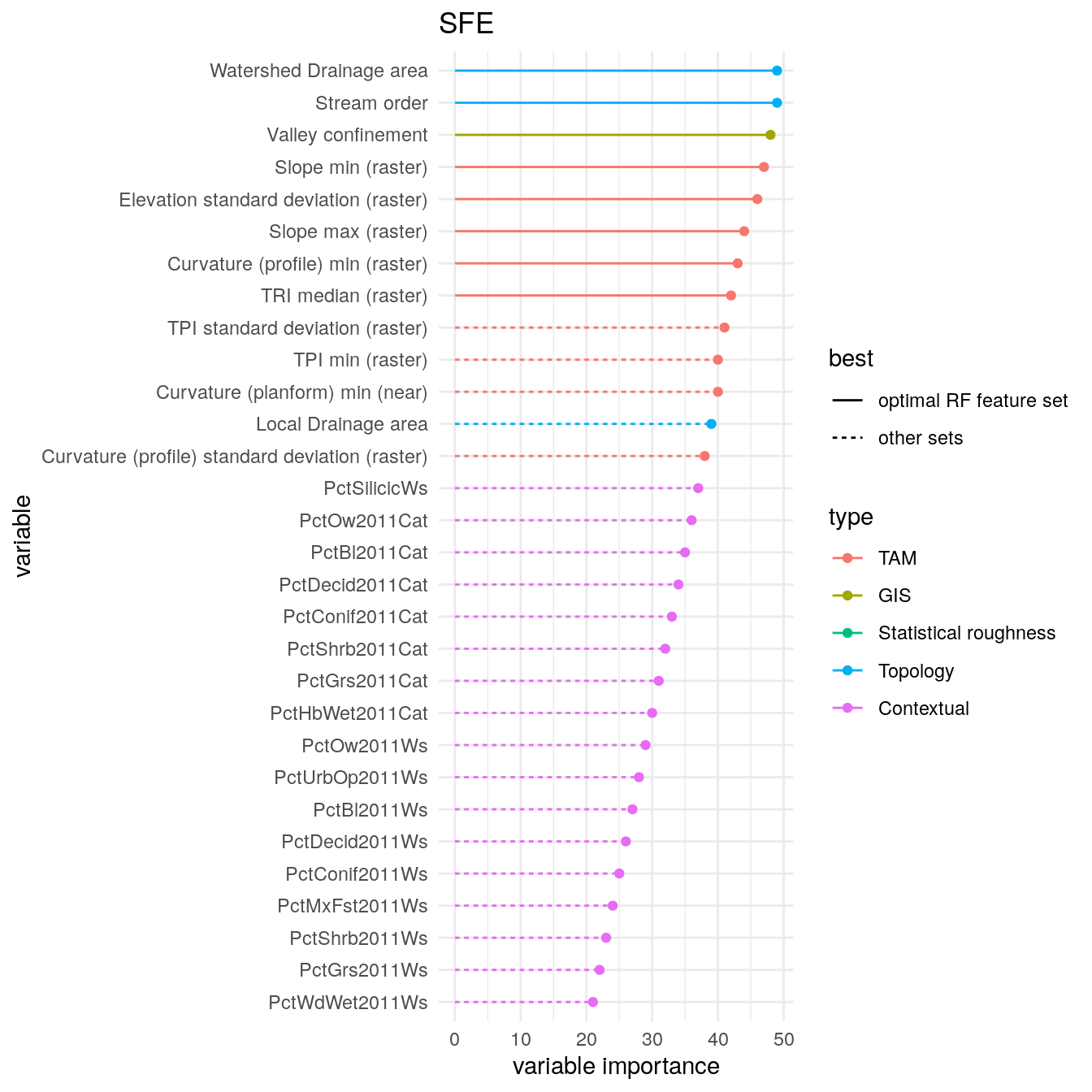
A convenience function, makeAllFeatureImportancePlotsFS(), creates all the feature importance plots from the standpoint of feature selection, that is evaluating which feature is present in the optimal feature sets. Here is an example for the SFE region.

FeatureImportancePlots <- makeAllFeatureImportancePlotFS(BMR_perf, selectedPATH, bestFeatureSets)
FeatureImportancePlots[["SFE"]]

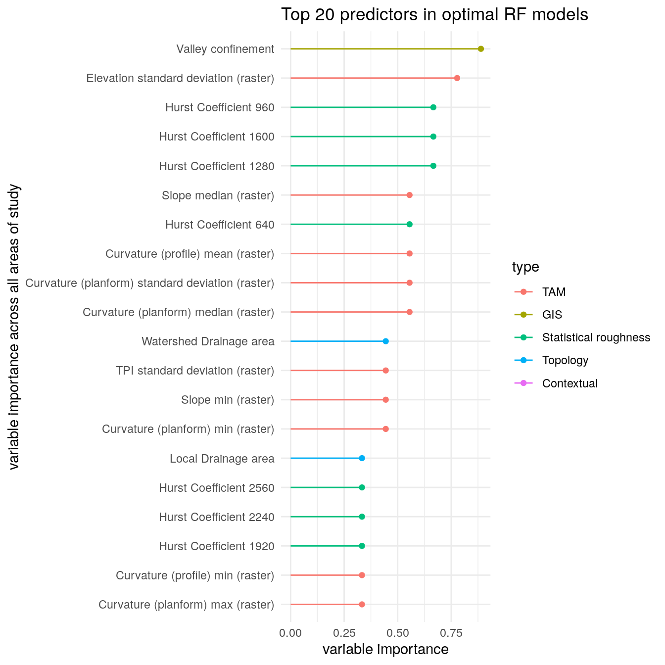
We can also investigate which features are often selected across all regions with getFreqBestFeatureSets().

freq_bestFeatureSets <- getFreqBestFeatureSets(bestFeatureSets)
freq_bestFeatureSets %>%
    dplyr::rename(var = group, Overall = prop) %>%
    dplyr::arrange(-Overall) %>%
    makeFeatureImportancePlot(first = 20) +
    ggplot2::labs(title = "Top 20 predictors in optimal RF models", y = "variable importance across all areas of study")

Performance of optimal models

We now turn to analyzing the tuning result contained in BMR_tune.

BMR_tune <- getBMR_perf_tune(BMR_res, type = "tune")
BMR_tune %>% dplyr::sample_n(10) %>%
    knitr::kable(digits = 3, format = "html", caption = "benchmark results") %>%
    kableExtra::kable_styling(bootstrap_options = c("hover", "condensed")) %>%
    kableExtra::scroll_box(width = "7in", height = "5in")

benchmark results
task.id	learner.id	iter	max.number.of.layers	hidden	activationfun	output	numepochs	learningrate	batchsize	momentum	hidden_dropout	visible_dropout	multiclass.au1u	acc	mmce	multiclass.aunu	timetrain	FS_NUM	mtry	cost	kernel
SFE	svm	22	NA	NA	NA	NA	NA	NA	NA	NA	NA	NA	0.963	0.841	0.159	0.959	0.085	41	NA	0.25	linear
SC	svm	65	NA	NA	NA	NA	NA	NA	NA	NA	NA	NA	0.928	0.764	0.236	0.910	0.037	18	NA	4.00	linear
NCC	svm	7	NA	NA	NA	NA	NA	NA	NA	NA	NA	NA	0.954	0.773	0.227	0.943	0.116	42	NA	1024.00	linear
SC	randomForest	4	NA	NA	NA	NA	NA	NA	NA	NA	NA	NA	0.866	0.592	0.408	0.819	0.083	3	3	NA	NA
NCC	randomForest	61	NA	NA	NA	NA	NA	NA	NA	NA	NA	NA	0.956	0.732	0.268	0.939	0.300	25	6	NA	NA
SCC	randomForest	35	NA	NA	NA	NA	NA	NA	NA	NA	NA	NA	0.934	0.669	0.331	0.916	0.142	4	2	NA	NA
SECA	randomForest	34	NA	NA	NA	NA	NA	NA	NA	NA	NA	NA	0.954	0.753	0.247	0.936	0.104	18	6	NA	NA
SCC	svm	49	NA	NA	NA	NA	NA	NA	NA	NA	NA	NA	0.918	0.568	0.432	0.873	1.000	11	NA	256.00	linear
SFE	nnTrain	80	2	30	tanh	softmax	20	0.05	16	0.8	0	0	0.969	0.812	0.188	0.960	0.806	18	NA	NA	NA
SECA	svm	9	NA	NA	NA	NA	NA	NA	NA	NA	NA	NA	0.902	0.470	0.530	0.830	0.096	3	NA	512.00	linear

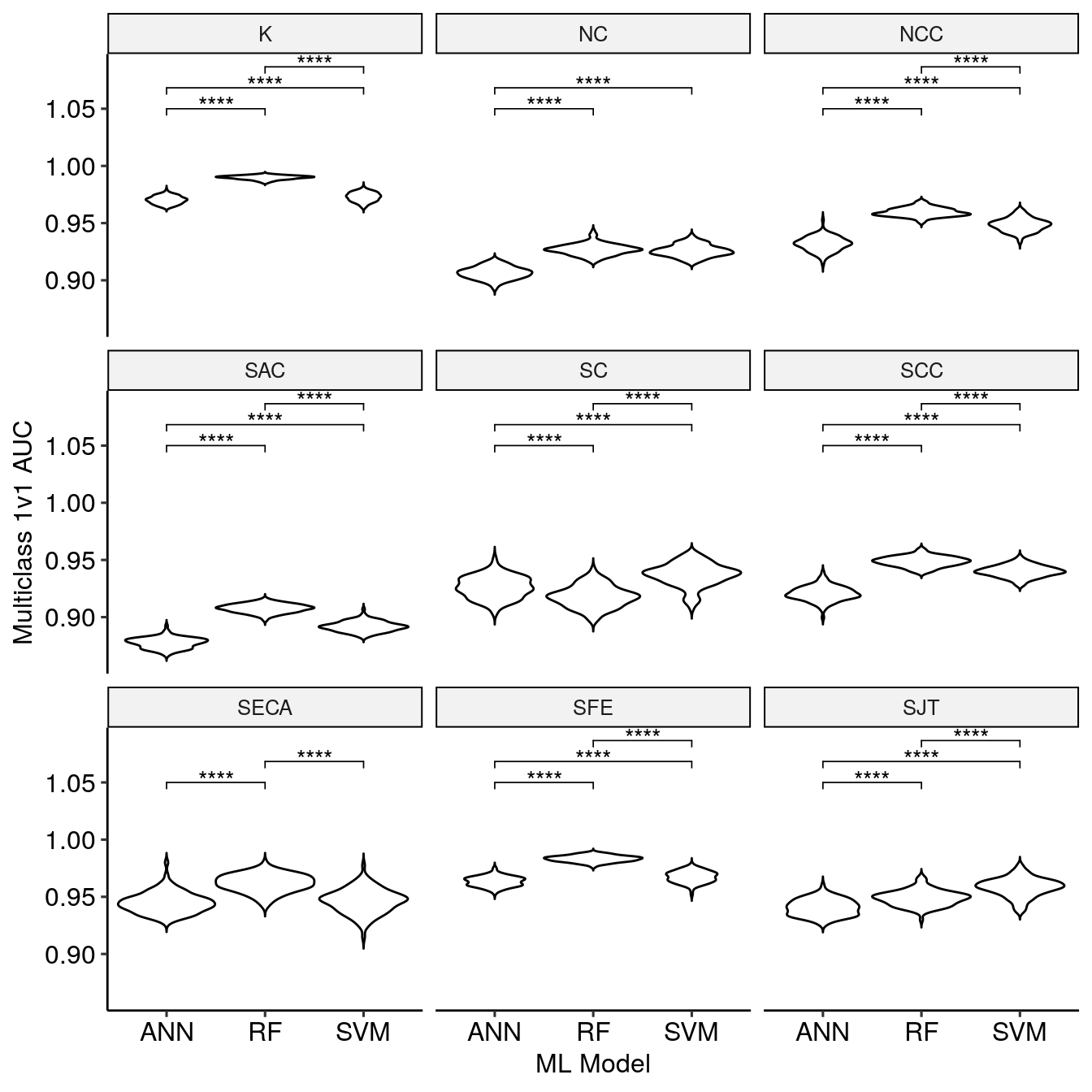
This data is subsetted by the optimal model selection with getBestBMRTune(). The resulting data.frame can be visualized with makeBestTuneAUCPlot() to compare the results of the optimal models.

bestBMR_tune <- getBestBMRTune(BMR_tune, bestFeatureSets)
makeBestTuneAUCPlot(bestBMR_tune)

Tuning entropy

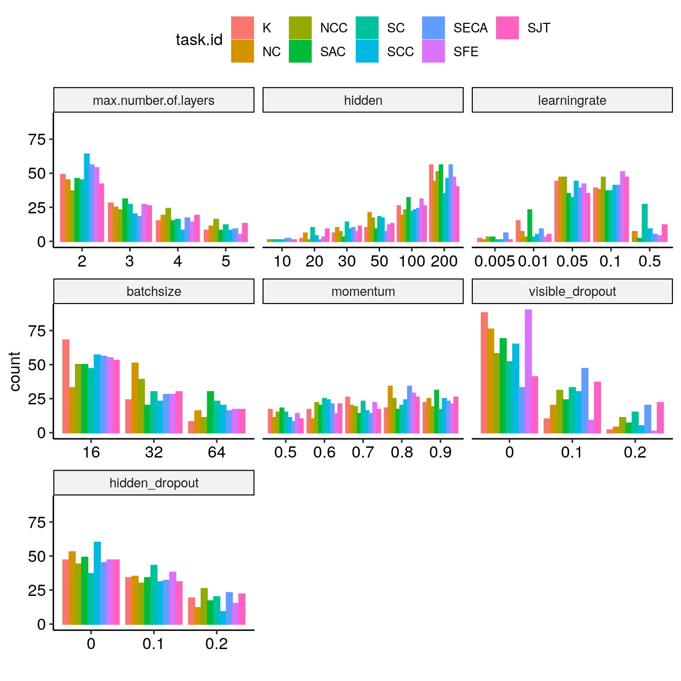
Because the benchmark used nested resampling, we have access to a distribution of best tune hyper-parameters which can be visualized with getTunePlot().

getTunePlot(bestBMR_tune, "nnTrain")

In addition, while the previous plot focused on the optimal, we can investigate how the tuning entropy evolves with the number of selected features using getBMRTuningEntropy(), getBestBMRTuningEntropy(), and makeTuningEntropyPlot(). Here is one example for the SFE region.

TUNELENGTH <- 16
BMR_lrnH <- getBMRTuningEntropy(BMR_tune, TUNELENGTH)
bestBMR_lrnH <- getBestBMRTuningEntropy(BMR_lrnH, bestFeatureSets, bestBMR_tune)
p_Hnorms <- makeTuningEntropyPlot(BMR_lrnH, bestBMR_lrnH)
p_Hnorms[["SFE"]]