LDA comparison

Purpose

In this vignette, we compare the topics outputted by topic modelling on three different corpora in English, Spanish and Porturguese.

Data loading

We access the topic lists stored in extdata using system.file().

library(dplyr)
library(reshape2)
en <- read.csv(system.file(
    "extdata",
    "topic_names_en.csv",
    package = "wateReview")
) %>% mutate(lang = "en") %>% melt(id.vars = c("topic_id","lang"))
es <- read.csv(system.file(
    "extdata",
    "topic_names_es.csv",
    package = "wateReview")
) %>% mutate(lang = "es") %>% melt(id.vars = c("topic_id","lang"))
pt <- read.csv(system.file(
    "extdata",
    "topic_names_pt.csv",
    package = "wateReview"),
    na.strings=c("","NA")
) %>% mutate(lang = "pt") %>% melt(id.vars = c("topic_id","lang"))

Each of these language data.frame holds the topic_id outputted by the topic model and a language identifier lang. variable holds the category of topics: general, specific, water budget, methods and theme and value the corresponding topic name.

head(en %>% filter(variable == "NSF_specific"))
#>   topic_id lang     variable                   value
#> 1       66   en NSF_specific  agricultural economics
#> 2       17   en NSF_specific agronomy & crop science
#> 3       34   en NSF_specific agronomy & crop science
#> 4       46   en NSF_specific agronomy & crop science
#> 5       55   en NSF_specific    analytical chemistry
#> 6        4   en NSF_specific          animal science

We now bind the three language data.frames, filter for the specific topics and count their occurence across themes per topic and language.

lda_comparison <- rbind(en, es, pt) %>% na.omit() %>%
  filter(variable == "NSF_specific") %>%
  group_by(value, lang) %>%
  tally()
head(lda_comparison)
#> # A tibble: 6 x 3
#> # Groups:   value [3]
#>   value                    lang      n
#>   <chr>                    <chr> <int>
#> 1 agricultural economics   en        1
#> 2 agricultural economics   pt        1
#> 3 agricultural engineering es        1
#> 4 agricultural engineering pt        2
#> 5 agronomy & crop science  en        3
#> 6 agronomy & crop science  es        1

To compare Spanish and Portuguese results with the English ones, we need to re-order the data.frame based on the tally of the English results and the overall number of covered topics.

lda_comparison$nlang <- lda_comparison %>%
  group_by(value) %>%
  group_map(~ rep(length(table(.x$lang)), length(table(.x$lang)))) %>%
  unlist()
lvls <- as.character(lda_comparison$value[lda_comparison$lang=="en"])[order(lda_comparison$n[lda_comparison$lang=="en"])]
lda_comparison$value <- factor(lda_comparison$value, levels = lvls)
lda_comparison <- na.omit(lda_comparison) # missing 1 spanish?
lda_comparison$lang <- factor(lda_comparison$lang, labels = c("English", "Spanish", "Portuguese"))

Visualization

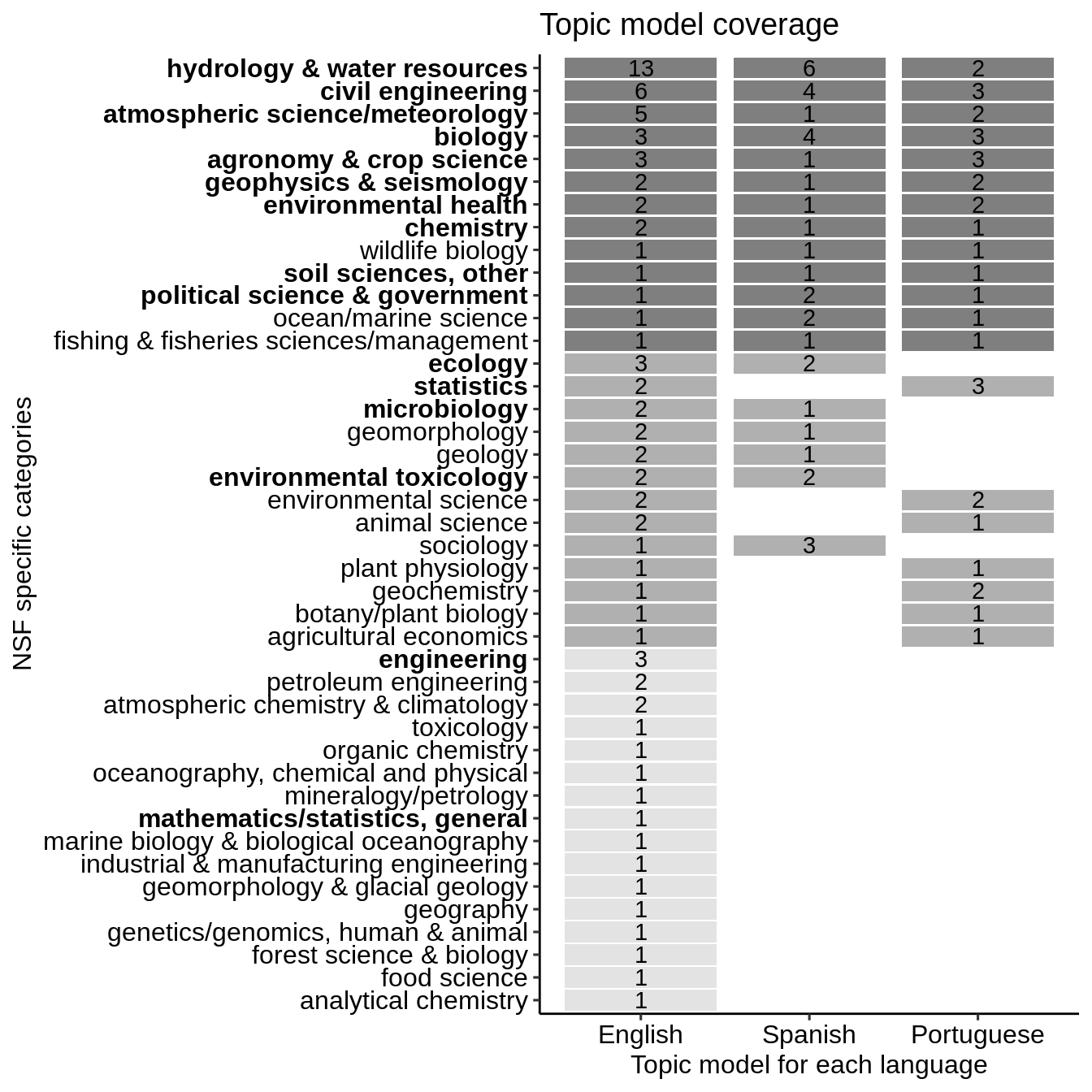
We now load some visualization libraries and presents the comparison as a heatmap where the number corresponds to the number of raw LDA topics and the color to the coverage between the three languages. Bold labels represent the top 12.5% specific research topics in terms of research volume across the corpus.

library(ggplot2)
library(forcats)
library(ggpubr)
ggplot(data = lda_comparison, aes(x = lang, y = fct_reorder(value, nlang))) +
  geom_tile(aes(fill = nlang, width=0.9, height=0.9)) +
  geom_text(aes(label = n)) +
  scale_fill_gradient(low = "grey89",
                      high = "grey50") +
  labs(title= "Topic model coverage",
       y="NSF specific categories",
       x = "Topic model for each language") +
  theme_pubr() +
  theme(axis.text.y = element_text(face = c('plain','plain','plain', 'plain', 'plain', 'plain', 'plain',
                                            'plain', 'bold', 'plain', 'plain', 'plain',
                                            'plain', 'plain', 'plain', 'bold', 'plain',
                                            'plain', 'plain', 'plain', 'plain', 'plain',
                                            'plain', 'bold', 'plain', 'plain', 'bold',
                                            'bold', 'bold', 'plain', 'plain', 'bold',
                                            'bold', 'plain', 'bold','bold', 'bold', # 6-10
                                            'bold', 'bold', 'bold','bold','bold' # 1-5
                                            ))) +
  rremove("legend")