Purpose

In this vignette, we derive the entropy at the country level for different categories of topics. Entropy describes how predictable a random variable \(X\) with discrete probability mass function \(P\) over \(n\) outcomes is (Shannon 1948):

\[ H(X) = - \sum_{i=1}^n P(x_i) log_b P(x_i)\]

In our case, \(P(x_i)\) represents the topic probabilities outputted by the topic model. In ecology, entropy is related to diversity through the Shannon-Wiener index. Diversity is used interchangeably with entropy in this vignette and in the function naming.

Data loading

We access the consolidated results stored in extdata using system.file().

general <- readRDS(system.file(
    "extdata",
    "consolidated_results_NSF_general.Rds",
    package = "wateReview")
)
specific <- readRDS(system.file(
    "extdata",
    "consolidated_results_NSF_specific.Rds",
    package = "wateReview")
)
methods <- readRDS(system.file(
    "extdata",
    "consolidated_results_methods.Rds",
    package = "wateReview")
)
budget <- readRDS(system.file(
    "extdata",
    "consolidated_results_water budget.Rds",
    package = "wateReview")
)
theme <-readRDS(system.file(
    "extdata",
    "consolidated_results_theme.Rds",
    package = "wateReview")
)

Calculating diversity

First, we attach the wateReview and dplyr packages.

library(wateReview)
library(dplyr)

Then, we calculate the diversity by paper and for all of LAC using the diversity_country() function, largely dependent on vegan::diversity().

relevant_documents <- remove_year_country(specific) #  specify which (species group)
diversity_LA <- diversity_LAC(relevant_documents)
diversity_paper <- vegan::diversity(relevant_documents)
general <- diversity_country(general)
specific <- diversity_country(specific)
budget <- diversity_country(budget)
diversity_by_country <- full_join(
    general,
    full_join(specific, budget, by = "country"),
    by = "country") %>%
   rename(general = x, specific = x.x, budget = x.y)

Here is the resulting table:

diversity_by_country %>% knitr::kable(digits = 3, align = "lccc", format = "html", caption = "Country entropy for general, specific and water budget topics") %>%
kableExtra::kable_styling(bootstrap_options = c("hover", "condensed"))

Country entropy for general, specific and water budget topics
country	general	specific	budget
Argentina	1.200	3.332	2.654
Belize	1.163	3.365	2.660
Bolivia	1.342	3.138	2.683
Brazil	1.306	3.320	2.676
Chile	1.276	3.354	2.701
Colombia	1.378	3.307	2.668
Costa.Rica	1.233	3.135	2.626
Ecuador	1.402	3.148	2.663
Mexico	1.281	3.321	2.690
Panama	1.195	3.099	2.530
Paraguay	1.345	2.903	2.283
Peru	1.294	3.261	2.619
Uruguay	1.275	3.333	2.642
Venezuela	1.206	3.393	2.664

Visualizing diversity with dot plots

To visualize the diversity, we attach some visualizations packages and prepare the data for visualization.

library(ggplot2)
library(ggpubr)
library(ggrepel)
library(reshape2)
diversity_by_country_graph <- melt(diversity_by_country, id.vars = c("country"))

Now, let’s visualize.

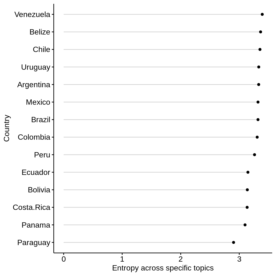
Specific topics

specific_graphdf <- subset(diversity_by_country_graph, variable == "specific")
specific_graph <- ggdotchart(specific_graphdf, x = "country", y = "value", #add color = cluster
                             add = "segments", sorting = "descending", rotate = TRUE,
                             ylab = "Entropy across specific topics",
                             xlab = "Country")
specific_graph

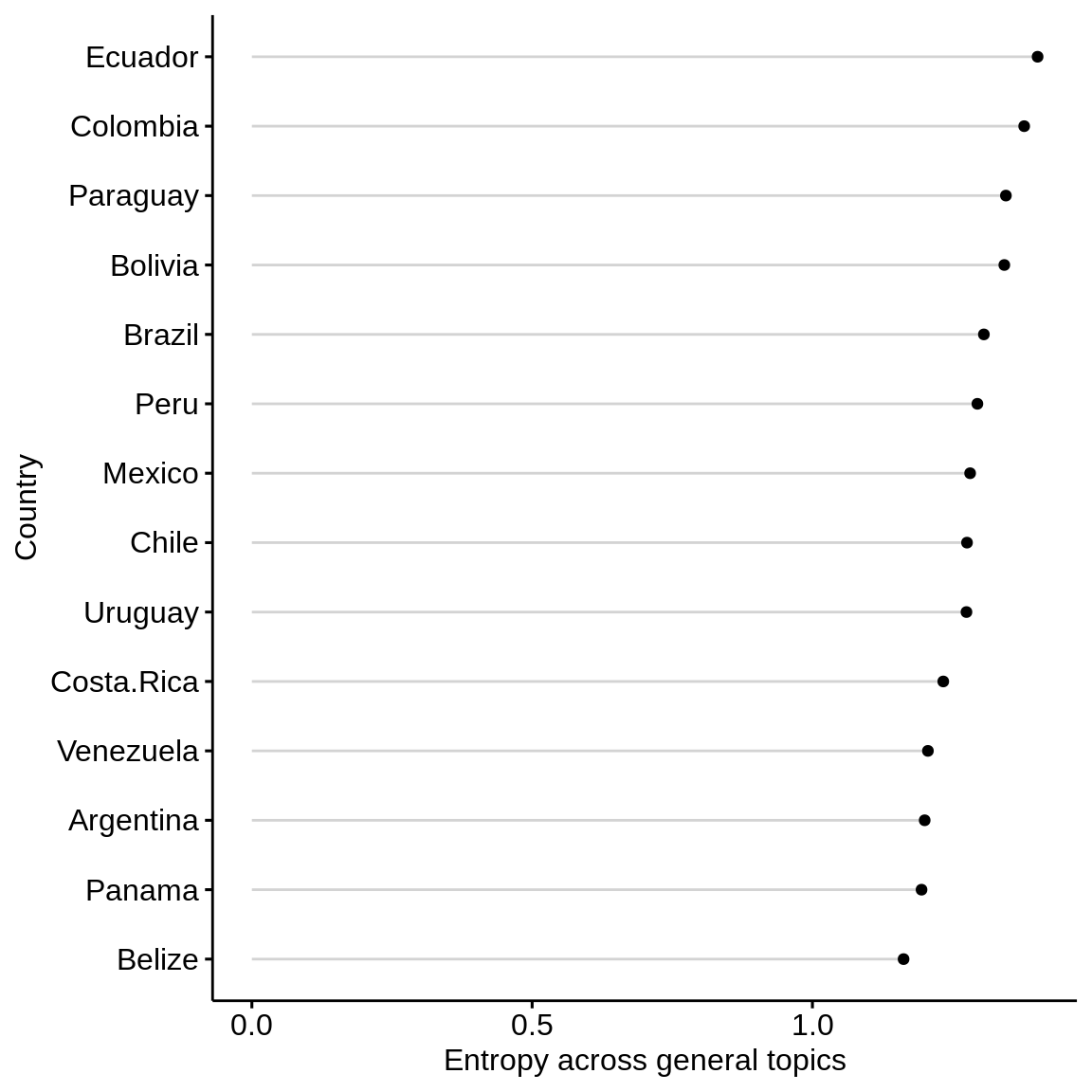
General topics

general_graphdf <- subset(diversity_by_country_graph, variable == "general")
general_graph <- ggdotchart(general_graphdf, x = "country", y = "value", #add color = cluster
                            add = "segments", sorting = "descending", rotate = TRUE,
                            ylab = "Entropy across general topics",
                            xlab = "Country")
general_graph

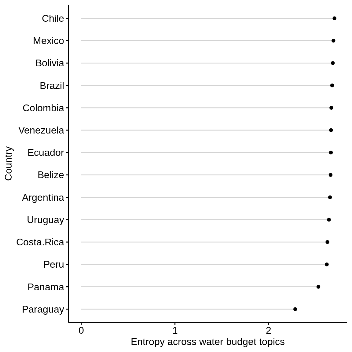
Water budget topics

budget_graphdf <- subset(diversity_by_country_graph, variable == "budget")
budget_graph <- ggdotchart(budget_graphdf, x = "country", y = "value", #add color = cluster
                             add = "segments", sorting = "descending", rotate = TRUE,
                           ylab = "Entropy across water budget topics",
                           xlab = "Country")

budget_graph

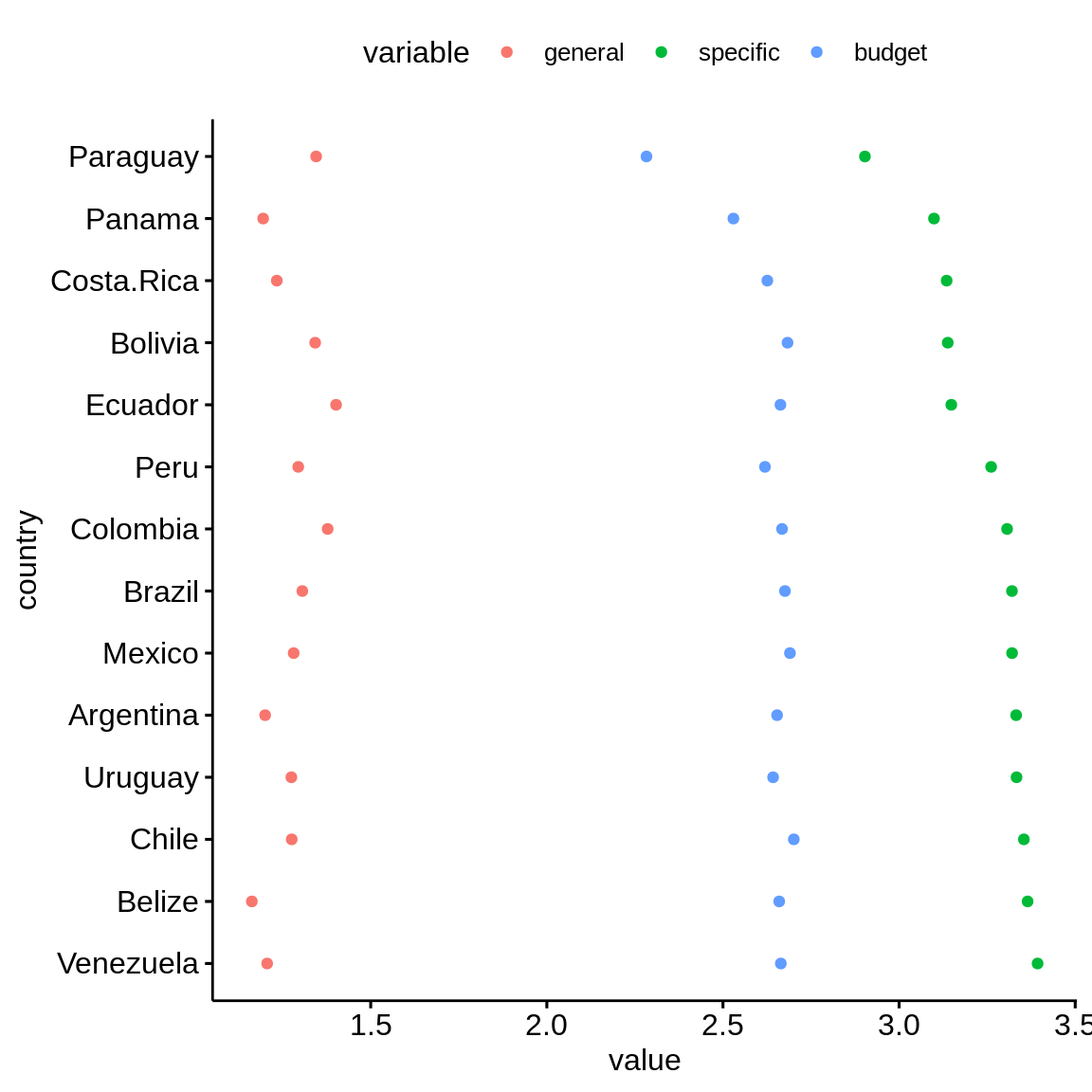
ggdotchart(diversity_by_country_graph, x = "country", y = "value", color = "variable",
           rotate = TRUE)

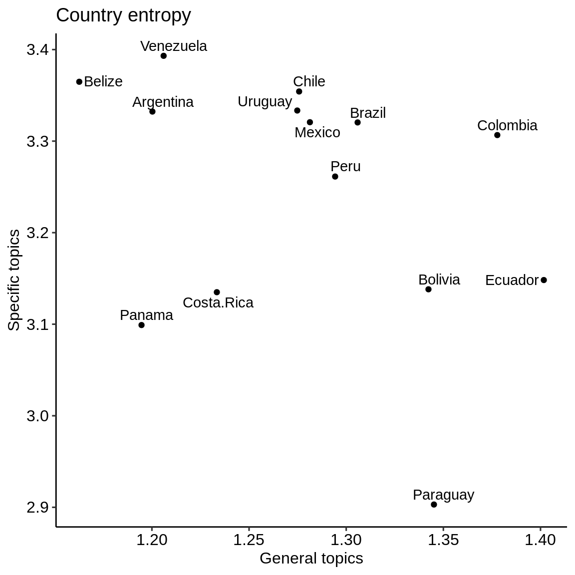
ggplot(diversity_by_country,aes(general, specific, label = country)) +
  geom_text_repel() +
  geom_point() +
  theme_pubr() +
  labs(x = "General topics",y = "Specific topics", title = "Country entropy")

References

Shannon, Claude Elwood. 1948. “A Mathematical Theory of Communication.” Bell System Technical Journal 27 (3). Wiley Online Library: 379–423. https://doi.org/10.1002/j.1538-7305.1948.tb01338.x.