ML predictions
ML_predictions.RmdLocation Prediction
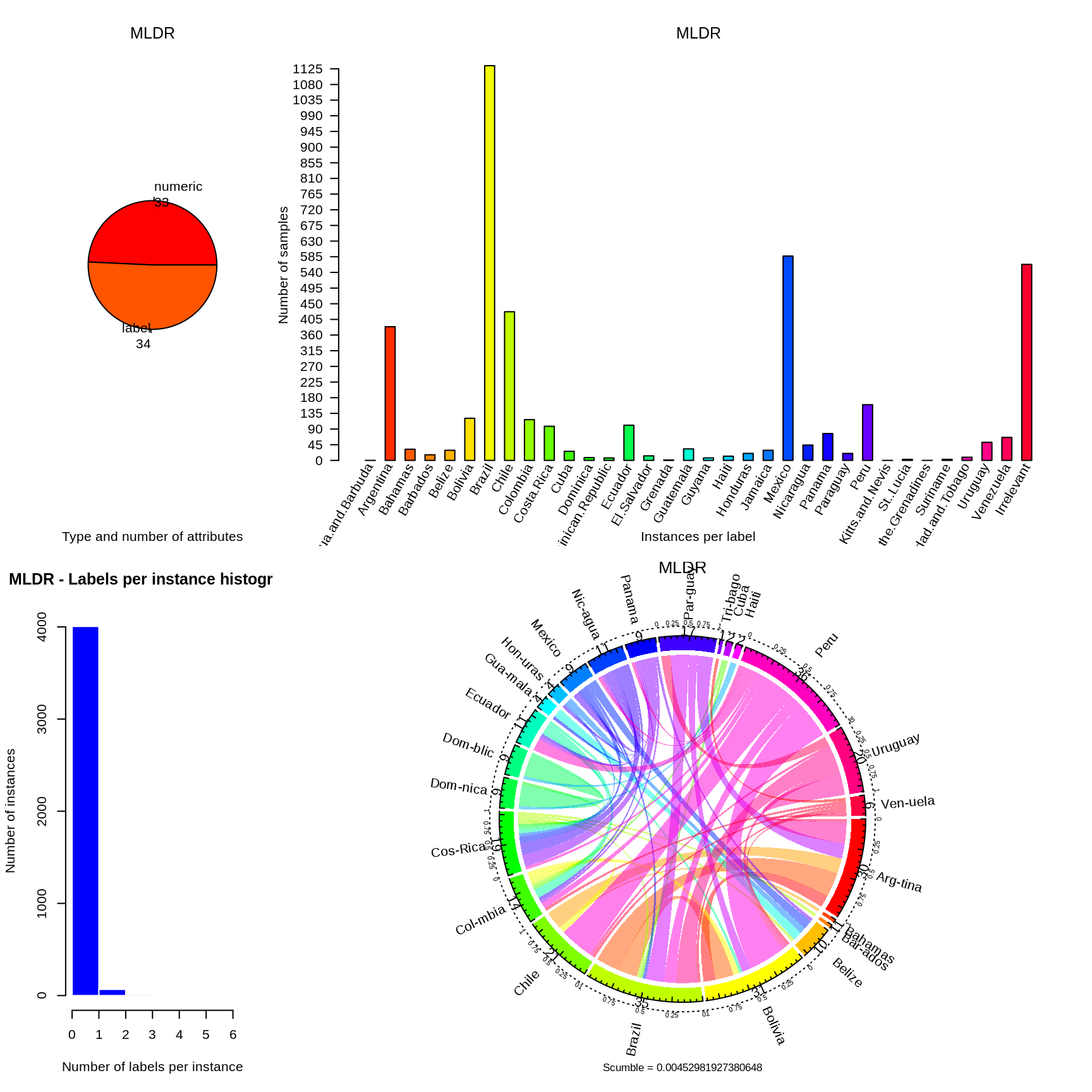
Machine learning predicts the location of the country of study of each paper. The training labels were provided by human-reading randomly chosen articles from the corpus (1,428 human-derived labels) and from text mining the article metadata (2,663 text-mined labels). Interestingly, the human-reading provided 563 observations of irrelevant country locations or irrelevant subjects of study.
The human-derived labels are first used for constructing a relevance filter based on simple binary classification between “Relevant” and “Irrelevant” documents (\(n = 1,386\)). The predictors consist of the text document term matrix derived from the cleaned corpus text using tokens related to country names and of the topic membership output by the topic model (\(p = 138\)). A benchmark of the six following models was conducted: featureless (baseline), random forest, support vector machine, naive Bayes, multinomial regression and extreme gradient boosting. The hyper-parameters are initially set at standard default value. The resampling scheme is 10 repeats of 10-fold cross-validation. The random forest, multinomal and support vector machine models are the best-performing model and show no statistical difference in the distribution of their performance measured by area-under-curve (AUC). These models are selected for further tuning using a nested cross-validation with a simple hold-out inner loop and 10 repeats of 10-fold cross-validation as outer loop. The size of the tuning grid is set to 16 between standard values for each hyper-parameters. Random forest and multinomial are the best-performing tuned models and show no statistical difference in the distribution of their performance measured by AUC. The distribution of the hyper-parameter resulting from the nested cross-validation shows a better constraint for the multinomial model and it is selected for predictions. The performance of such multinomial model corresponds to a mean AUC of 0.82, a mean accuracy of 77% and a true positive rate of 86%.
The prediction of the location of study for each document is performed using both human-derived and text-mined labels (\(n = 3,494\)). The predictors consist of the text document term matrix derived from the cleaned corpus text using tokens related to country names (\(p = 33\)). Models and resampling scheme are similar than the ones used for the relevance filter. The hyper-parameters are initially set at standard default value. Random forest outperforms every other model with a mean multiclass AUC of 0.99 and a mean accuracy of 96%. No further tuning is performed and the random forest with default hyper-parameters is used for predictions. More complex approaches were investigated: using additional geographical tokens (e.g. rivers and mountain ranges names), multilabel classifications (e.g. binary relevance, label powerset) or deep learning models of natural language processing (e.g. BERT) both on full texts and abstracts with little benefits.
Libraries
library(wateReview)
Defining parameters
SCALE_TYPE <- "location"
MODEL_TYPE <- "multiclass" # multiclass or binary_relevance
AGGREGATE <- FALSE
Data reading
topicDocs <- get_topicDocs()
titleDocs <- get_titleDocs(topicDocs)
validationHumanReading <-  get_validationHumanReading(scale_type = SCALE_TYPE)
DTM <- get_DocTermMatrix()
webscrapped_validationDTM <- get_webscrapped_validationDTM()
colnames(webscrapped_validationDTM) <- colnames(DTM)
#> Loading required package: quanteda
#> Package version: 2.1.1
#> Parallel computing: 2 of 2 threads used.
#> See https://quanteda.io for tutorials and examples.
#>
#> Attaching package: 'quanteda'
#> The following object is masked from 'package:utils':
#>
#>     View
webscrapped_validationDTM <- transform_DTM(webscrapped_validationDTM)
DTM <- transform_DTM(DTM)
webscrapped_trainingLabels <- get_webscrapped_trainingLabels()
titleInd <- get_titleInd(humanReadingDatabase = validationHumanReading, topicModelTitles = titleDocs)
Sanity check
We now check if all the papers are found, address issues and align databases.
table(is.na(titleInd))
#>
#> FALSE  TRUE
#>  1430   121
alignedData <- align_humanReadingTopicModel(titleInd, validationHumanReading, topicDocs, DTM)
alignedData <- QA_alignedData(alignedData, scale_type = SCALE_TYPE)
validationTopicDocs <- alignedData$validationTopicDocs
validationHumanReading <- alignedData$validationHumanReading
validationHumanReadingDTM <- alignedData$validationDTM
Get the training data from humanReadingTrainingLabels
humanReadingTrainingLabels <- make_humanReadingTrainingLabels(validationHumanReading, scale_type = SCALE_TYPE, webscrapped_trainingLabels)
#> [1] "These labels are missing from the human read labels:"
#>  [1] "Antigua.and.Barbuda"            "Cuba"
#>  [3] "Dominica"                       "Dominican.Republic"
#>  [5] "Grenada"                        "Guyana"
#>  [7] "St..Kitts.and.Nevis"            "St..Lucia"
#>  [9] "St..Vincent.and.the.Grenadines" "Suriname"
trainingData <- make_trainingData(validationHumanReadingDTM, humanReadingTrainingLabels, webscrapped_validationDTM, webscrapped_trainingLabels, scale_type = SCALE_TYPE, aggregate_labels = AGGREGATE)
head(trainingData, 5) %>%
    knitr::kable(digits = 3, format = "html", caption = "") %>%
    kableExtra::kable_styling(bootstrap_options = c("hover", "condensed")) %>%
    kableExtra::scroll_box(width = "7in")
| Term1 | Term2 | Term3 | Term4 | Term5 | Term6 | Term7 | Term8 | Term9 | Term10 | Term11 | Term12 | Term13 | Term14 | Term15 | Term16 | Term17 | Term18 | Term19 | Term20 | Term21 | Term22 | Term23 | Term24 | Term25 | Term26 | Term27 | Term28 | Term29 | Term30 | Term31 | Term32 | Term33 | Antigua.and.Barbuda | Argentina | Bahamas | Barbados | Belize | Bolivia | Brazil | Chile | Colombia | Costa.Rica | Cuba | Dominica | Dominican.Republic | Ecuador | El.Salvador | Grenada | Guatemala | Guyana | Haiti | Honduras | Jamaica | Mexico | Nicaragua | Panama | Paraguay | Peru | St..Kitts.and.Nevis | St..Lucia | St..Vincent.and.the.Grenadines | Suriname | Trinidad.and.Tobago | Uruguay | Venezuela | Irrelevant | |
|---|---|---|---|---|---|---|---|---|---|---|---|---|---|---|---|---|---|---|---|---|---|---|---|---|---|---|---|---|---|---|---|---|---|---|---|---|---|---|---|---|---|---|---|---|---|---|---|---|---|---|---|---|---|---|---|---|---|---|---|---|---|---|---|---|---|---|---|
| 13816 | 0 | 1 | 0 | 0 | 0 | 0 | 1 | 1 | 1 | 0 | 0 | 2 | 0 | 0 | 0 | 0 | 0 | 0 | 0 | 0 | 0 | 0 | 0 | 0 | 0 | 3 | 0 | 0 | 0 | 0 | 0 | 0 | 1 | FALSE | FALSE | FALSE | FALSE | FALSE | FALSE | FALSE | FALSE | FALSE | FALSE | FALSE | FALSE | FALSE | FALSE | FALSE | FALSE | FALSE | FALSE | FALSE | FALSE | FALSE | FALSE | FALSE | FALSE | FALSE | FALSE | FALSE | FALSE | FALSE | FALSE | FALSE | FALSE | FALSE | TRUE |
| 527 | 0 | 0 | 0 | 0 | 0 | 0 | 0 | 39 | 0 | 3 | 0 | 0 | 0 | 0 | 0 | 0 | 0 | 0 | 0 | 0 | 0 | 0 | 0 | 0 | 0 | 0 | 0 | 0 | 0 | 0 | 0 | 0 | 0 | FALSE | FALSE | FALSE | FALSE | FALSE | FALSE | FALSE | FALSE | FALSE | FALSE | FALSE | FALSE | FALSE | FALSE | FALSE | FALSE | FALSE | FALSE | FALSE | FALSE | FALSE | FALSE | FALSE | FALSE | FALSE | FALSE | FALSE | FALSE | FALSE | FALSE | FALSE | FALSE | FALSE | TRUE |
| 7597 | 0 | 0 | 0 | 0 | 0 | 0 | 16 | 0 | 0 | 0 | 0 | 0 | 0 | 0 | 0 | 0 | 0 | 0 | 0 | 0 | 0 | 0 | 0 | 0 | 0 | 0 | 0 | 0 | 0 | 0 | 0 | 0 | 0 | FALSE | FALSE | FALSE | FALSE | FALSE | FALSE | TRUE | FALSE | FALSE | FALSE | FALSE | FALSE | FALSE | FALSE | FALSE | FALSE | FALSE | FALSE | FALSE | FALSE | FALSE | FALSE | FALSE | FALSE | FALSE | FALSE | FALSE | FALSE | FALSE | FALSE | FALSE | FALSE | FALSE | FALSE |
| 2857 | 0 | 2 | 0 | 0 | 0 | 41 | 0 | 0 | 0 | 1 | 0 | 0 | 1 | 0 | 0 | 0 | 0 | 1 | 0 | 0 | 0 | 0 | 0 | 0 | 0 | 0 | 0 | 0 | 0 | 0 | 0 | 0 | 0 | FALSE | FALSE | FALSE | FALSE | FALSE | TRUE | FALSE | FALSE | FALSE | FALSE | FALSE | FALSE | FALSE | FALSE | FALSE | FALSE | FALSE | FALSE | FALSE | FALSE | FALSE | FALSE | FALSE | FALSE | FALSE | FALSE | FALSE | FALSE | FALSE | FALSE | FALSE | FALSE | FALSE | FALSE |
| 5379 | 0 | 0 | 0 | 0 | 0 | 0 | 0 | 0 | 0 | 0 | 0 | 0 | 0 | 0 | 0 | 0 | 0 | 0 | 0 | 0 | 0 | 4 | 0 | 0 | 0 | 0 | 0 | 0 | 0 | 0 | 0 | 0 | 0 | FALSE | FALSE | FALSE | FALSE | FALSE | FALSE | FALSE | FALSE | FALSE | FALSE | FALSE | FALSE | FALSE | FALSE | FALSE | FALSE | FALSE | FALSE | FALSE | FALSE | FALSE | FALSE | FALSE | FALSE | FALSE | FALSE | FALSE | FALSE | FALSE | FALSE | FALSE | FALSE | FALSE | TRUE |
Exploratory data analysis
EDA_trainingData(trainingData, validationHumanReadingDTM, humanReadingTrainingLabels) %>%
    knitr::kable(digits = 3, format = "html", caption = "") %>%
    kableExtra::kable_styling(bootstrap_options = c("hover", "condensed")) %>%
    kableExtra::scroll_box(width = "7in", height = "7in")
| country | human_reading | human_reading_webscrapping | webscrapping |
|---|---|---|---|
| Antigua.and.Barbuda | 0 | 0 | 0 |
| Argentina | 104 | 384 | 280 |
| Bahamas | 6 | 32 | 26 |
| Barbados | 4 | 16 | 12 |
| Belize | 6 | 29 | 23 |
| Bolivia | 19 | 121 | 102 |
| Brazil | 372 | 1134 | 762 |
| Chile | 89 | 427 | 338 |
| Colombia | 26 | 117 | 91 |
| Costa.Rica | 14 | 98 | 84 |
| Cuba | 0 | 26 | 26 |
| Dominica | 0 | 8 | 8 |
| Dominican.Republic | 0 | 7 | 7 |
| Ecuador | 14 | 101 | 87 |
| El.Salvador | 2 | 13 | 11 |
| Grenada | 0 | 1 | 1 |
| Guatemala | 3 | 33 | 30 |
| Guyana | 0 | 7 | 7 |
| Haiti | 2 | 12 | 10 |
| Honduras | 3 | 20 | 17 |
| Jamaica | 5 | 29 | 24 |
| Mexico | 138 | 587 | 449 |
| Nicaragua | 5 | 44 | 39 |
| Panama | 11 | 77 | 66 |
| Paraguay | 4 | 20 | 16 |
| Peru | 35 | 160 | 125 |
| St..Kitts.and.Nevis | 0 | 0 | 0 |
| St..Lucia | 0 | 3 | 3 |
| St..Vincent.and.the.Grenadines | 0 | 0 | 0 |
| Suriname | 0 | 3 | 3 |
| Trinidad.and.Tobago | 5 | 9 | 4 |
| Uruguay | 14 | 52 | 38 |
| Venezuela | 15 | 66 | 51 |
| Irrelevant | 563 | 563 | 0 |
Multilabel: binary relevance and algorithm adaptation
The following code executes a multilabl benchmark.
bmr <- multilabelBenchmark(trainingData, validationHumanReadingDTM, MODEL_TYPE, scale_type = SCALE_TYPE, aggregated_labels = AGGREGATE, obs_threshold = 10)
AggrPerformances <- getBMRAggrPerformances(bmr, as.df = TRUE)
PerfVisMultilabel(AggrPerformances)
Multiclass
Relevance filter
trainingDataMulticlassFilter <- make_trainingDataMulticlass(trainingData, validationHumanReadingDTM, humanReadingTrainingLabels, webscrapped_validationDTM, webscrapped_trainingLabels,
    filter = TRUE,
    addTopicDocs = TRUE,
    validationTopicDocs = validationTopicDocs)
Selecting a model to tune
if (!file.exists("bmr_filter.Rds")){
    bmr_filter <- multiclassBenchmark(trainingDataMulticlassFilter, MODEL_TYPE, filter = TRUE)
    saveRDS(bmr_filter, "bmr_filter.Rds")
} else {
    bmr_filter <- readRDS("bmr_filter.Rds")
}
make_AUCPlot(bmr_filter, binary = TRUE)
Based on the result of the AUC plot comparison, svm, multinom and RF are selected for tuning benchmark
Tuning model
if(!file.exists("bmr_tune_filter.Rds")){
    bmr_tune_filter <- multiclassBenchmark(trainingDataMulticlassFilter, MODEL_TYPE, filter = TRUE, tune = list("classif.svm", "classif.randomForest", "classif.multinom"))
    saveRDS(bmr_tune_filter, "bmr_tune_filter.Rds")
} else {
    bmr_tune_filter <- readRDS("bmr_tune_filter.Rds")
}
make_AUCPlot(bmr_tune_filter, binary = TRUE)
RF and multninomal have similar performance, we pick multinom (better hyper-parameter constrains).
Country
trainingDataMulticlass <- make_trainingDataMulticlass(trainingData, validationHumanReadingDTM, humanReadingTrainingLabels, webscrapped_validationDTM, webscrapped_trainingLabels, filter = FALSE, addWebscrapped = TRUE)Selecting a model to tune
if (!file.exists("bmr_country.Rds")){
    bmr_country <- multiclassBenchmark(trainingDataMulticlass, MODEL_TYPE, filter = FALSE)
    saveRDS(bmr_country, "bmr_country.Rds")
} else {
    bmr_country <- readRDS("bmr_country.Rds")
}
make_AUCPlot(bmr_country)
Tuning
# bmr_tune_country <- multiclassBenchmark(trainingDataMulticlass, MODEL_TYPE, filter = FALSE, tune = list("classif.randomForest"))
# make_AUCPlot(bmr_tune_country)
# saveRDS(bmr_tune_country, "bmr_tune_country.Rds")
Predicting
targetData <- make_targetData(DTM)
predCountry <- make_predictions("classif.randomForest",
    list(mtry = floor(sqrt(ncol(trainingDataMulticlass) - 1))),
    trainingDataMulticlass, targetData, MODEL_TYPE, filter = FALSE)

predCountry$response <- as.character(predCountry$response)
predCountry$response[as.character(predRelevance) == "Irrelevant"] <- "Irrelevant"
predCountry$response <- as.factor(predCountry$response)

saveRDS(predRelevance, "predRelevance.Rds")
saveRDS(predCountry, "predCountry.Rds")
Consolidating results
We now consolidate all results to be used for analysis. Because this uses the complete corpus, the following code is not executed.
Cross-walk between databases
The following code chunks perform a cross-walk between the topic model and EndNote databases using document id: EndNoteIdcorpus and EndNoteIdLDA. This ensures that the two databases can communicate and are aligned.
Data loading
englishCorpus_file <- "F:/hguillon/research/exploitation/R/latin_america/data/english_corpus.Rds"
englishCorpus <- readRDS(englishCorpus_file)

in_corpus_file <- "in_corpus.Rds"
in_corpus <- readRDS(in_corpus_file)

predCountry <- readRDS("predCountry.Rds") # aligned with englishCorpus
predRelevance <- readRDS("predRelevance.Rds") # aligned with englishCorpus
topicDocs <- readRDS("./data/topicDocs.Rds") # aligned with englishCorpus
Get document IDs
EndNoteIdcorpus <- get_EndNoteIdcorpus(in_corpus)
EndNoteIdLDA <- get_EndNoteIdLDA(englishCorpus)
QA_EndNoteIdCorpusLDA(EndNoteIdLDA, EndNoteIdcorpus)
Align databases
in_corpus <- align_dataWithEndNoteIdcorpus(in_corpus, EndNoteIdcorpus, EndNoteIdLDA)

englishCorpus <- align_dataWithEndNoteIdLDA(englishCorpus, EndNoteIdLDA, EndNoteIdcorpus)
predCountry <- align_dataWithEndNoteIdLDA(predCountry, EndNoteIdLDA, EndNoteIdcorpus)
predRelevance <- align_dataWithEndNoteIdLDA(predRelevance, EndNoteIdLDA, EndNoteIdcorpus)
topicDocs <- align_dataWithEndNoteIdLDA(topicDocs, EndNoteIdLDA, EndNoteIdcorpus)

EndNoteIdLDA <- align_dataWithEndNoteIdLDA(EndNoteIdLDA, EndNoteIdLDA, EndNoteIdcorpus)
EndNoteIdcorpus <- align_dataWithEndNoteIdcorpus(EndNoteIdcorpus, EndNoteIdcorpus, EndNoteIdLDA)

QA_EndNoteIdCorpusLDA(EndNoteIdLDA, EndNoteIdcorpus)Saving results
saveRDS(predRelevance, "predRelevance.Rds")
saveRDS(predCountry %>% pull(response), "predCountry.Rds")
saveRDS(predCountry %>% select(-response), "predCountryMembership.Rds")
consolidate_LDA_results(theme_type = "topic_name", save = TRUE)
consolidate_LDA_results(theme_type = "theme", save = TRUE)
consolidate_LDA_results(theme_type = "NSF_general", save = TRUE)
consolidate_LDA_results(theme_type = "NSF_specific", save = TRUE)
consolidate_LDA_results(theme_type = "theme", description = "water budget", save = TRUE)
consolidate_LDA_results(theme_type = "theme", description = "methods", save = TRUE)
consolidate_LDA_results(theme_type = "theme", description = "spatial scale", save = TRUE)