Hexagonal maps of country entropies

Purpose

This vignette visualizes the country entropy.

Libraries

library(wateReview)
library(raster)
library(tmap)
library(geogrid)
library(RColorBrewer)
library(scales)

Data loading

We read a shapefile of the region with the country long and short names, the information from the English topics and the country entropy. We then min-max rescale the data so that each entropy, \(H\), is mapped following:

\[(0, \max H) \to (0,1)\]

These min-max rescaled data are assigned to the shapefile.

LAC_map <- shapefile(system.file("extdata", "LAC_di.shp", package = "wateReview"))
LAC_map@data <- subset(LAC_map@data, select = c("COUNTRY", "NAME"))
topics <- read.csv(system.file("extdata", "topic_names_en.csv", package = "wateReview"))
entropy_data <- read.csv(system.file("extdata", "diversity.csv", package = "wateReview"))
entropy_data$NSFgeneral <- scales::rescale(
  entropy_data$NSFgeneral,
  to = c(0, 1),
  from = c(0,  log(length(unique(topics$NSF_general)))))
entropy_data$NSFspecific <- scales::rescale(
  entropy_data$NSFspecific,
  to = c(0, 1),
  from = c(0,  log(length(unique(topics$NSF_specific)))))
entropy_data$budget <- scales::rescale(
  entropy_data$budget,
  to = c(0, 1),
  from = c(0,  log(nrow(topics[topics$description == "methods", ]))))
LAC_map <- LAC_map[LAC_map$COUNTRY %in% entropy_data$country, ]
LAC_map@data <- merge(LAC_map@data, entropy_data,  by.x= "COUNTRY", by.y = "country")

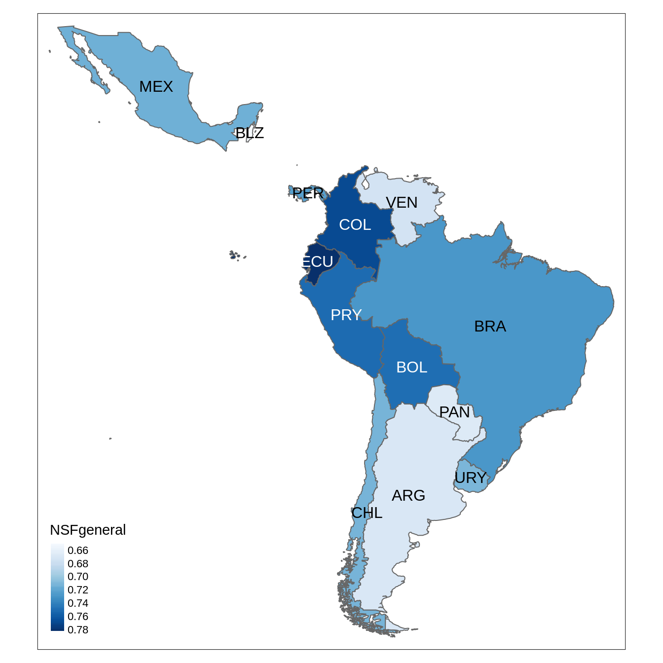
Non-hexagonal map

tm_shape(LAC_map) +
  tm_polygons("NSFgeneral", style = "cont", palette = "Blues") +
  tmap_options(max.categories = 50) +
  tm_text("NAME")

Generating hexagons

We use here the package geogrid.

LAC_hex <- assign_polygons(LAC_map, calculate_grid(shape = LAC_map, grid_type = "hexagonal", seed = 5))

Hexagonal maps

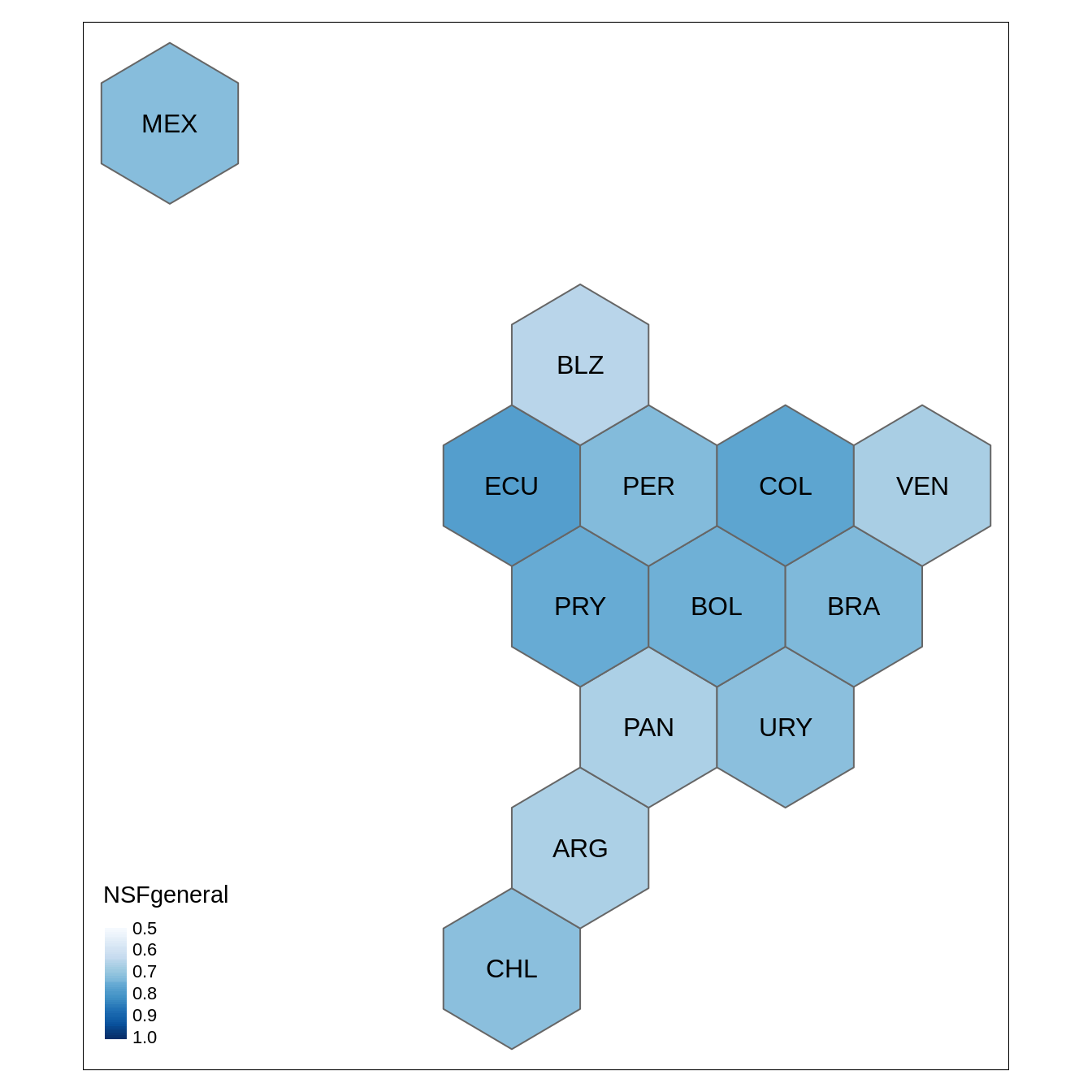
General topics

pal <- "Blues"
brk <- seq(.5, 1, by = .1)
tm_shape(LAC_hex) +
  tm_polygons("NSFgeneral", style = "cont", breaks = brk, palette = pal) +
  tm_text("NAME")

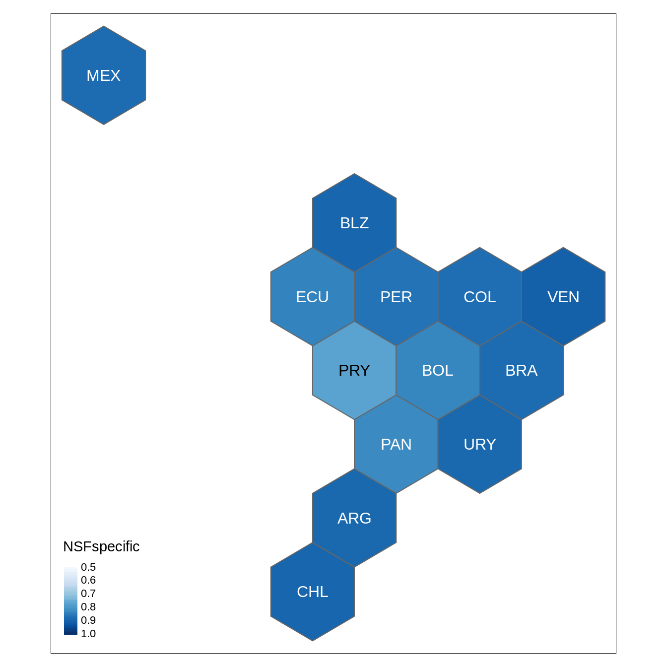
Specific topics

tm_shape(LAC_hex) +
  tm_polygons("NSFspecific", style = "cont", breaks = brk, palette = pal) +
  tm_text("NAME")

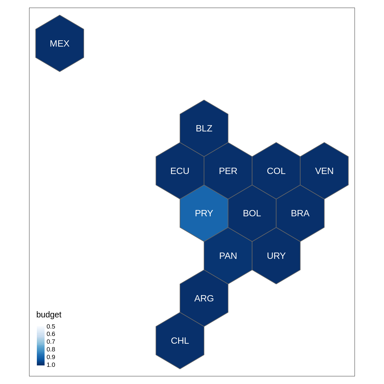
Water budget topics

tm_shape(LAC_hex) +
  tm_polygons("budget", style = "cont", breaks = brk, palette = pal) +
  tm_text("NAME")

This maps can these easily be modified with a vector drawing software.