Timelines
timelines.RmdData loading
We load the consolidated results for the entire corpus which contains the general topics caterogy and the predicted country.
documents_year_location <- readRDS(system.file("extdata", "consolidated_results_NSF_general.Rds", package = "wateReview")) %>%
  select(c(year, country)) %>%
  filter(country != "Irrelevant") %>%
  mutate(country = as.character(country))
dim(documents_year_location)
#> [1] 12616     2
head(documents_year_location)
#>   year   country
#> 1 2011    Mexico
#> 2 2005  Colombia
#> 3 1992 Venezuela
#> 4 2016 Argentina
#> 5 2015     Chile
#> 6 2015    Brazil
We group the country by clusters. We define a convenience function to do so which assign the country cluster to country and take care of removing the the Carribean countries which were not clustered.
assign_cluster <- function(country){
  cluster1 <- c("Mexico", "Brazil")
  cluster2 <- c("Chile", "Argentina", "Uruguay", "Suriname", "Guyana", "Belize", "Paraguay", "Costa.Rica", "Cuba", "Panama", "Venezuela")
  cluster3 <- c("Colombia", "Bolivia", "Jamaica", "Nicaragua", "El.Salvador", "Ecuador", "Honduras", "Guatemala", "Peru", "Dominican Republic")
  if (country %in% cluster1){
    return(1)
  } else if (country %in% cluster2){
    return(2)
  } else if (country %in% cluster3){
    return(3)
  } else {
    return(NA)
  }
}
documents_year_location <- documents_year_location %>%
  mutate(cluster = sapply(country, assign_cluster)) %>%
  na.omit()
dim(documents_year_location)
#> [1] 12615     3
head(documents_year_location)
#>   year   country cluster
#> 1 2011    Mexico       1
#> 2 2005  Colombia       3
#> 3 1992 Venezuela       2
#> 4 2016 Argentina       2
#> 5 2015     Chile       2
#> 6 2015    Brazil       1
Counting documents per year per cluster
count_year_cluster <- documents_year_location %>%
  select(-country) %>%
  group_by(cluster) %>%
  group_modify(~ table(.) %>% t() %>% as.data.frame()) %>%
  select(- Var1) %>%
  rename(year = ".", count = Freq) %>%
  mutate(cluster = as.factor(cluster), year = as.numeric(as.character(year))) %>%
  filter(year >= 2000) %>%
  filter(year < 2018) %>%
  tidyr::complete(year = tidyr::full_seq(year, period = 1))
 count_year_cluster$count[is.na(count_year_cluster$count)] <- 0
head(count_year_cluster)
#> # A tibble: 6 x 3
#> # Groups:   cluster [1]
#>   cluster  year count
#>   <fct>   <dbl> <dbl>
#> 1 1        2000    77
#> 2 1        2001   104
#> 3 1        2002   152
#> 4 1        2003   125
#> 5 1        2004   160
#> 6 1        2005   170
Visualizing growth through time
growth <- ggplot(count_year_cluster, aes(x = year, y = count, fill = cluster)) +
  theme_pubr(legend = "none") +
  geom_area(alpha = 0.6 , size =.5, colour = "white") +
  scale_fill_manual(
    values = c("#F8766D", "#00BFC4", "#7CAE00"),
    labels = c("Cluster 1", "Cluster 2", "Cluster 3")
    ) +
  scale_x_continuous(
    minor_breaks = seq(1980, 2020, by = 1),
    breaks = seq(1980, 2020, by = 5)
    ) +
  theme(
    axis.title.x = element_blank(),
    plot.title = element_text(hjust = 0.5),
    legend.title=element_blank()
    ) +
  labs(y = "New water resources articles", x = "Time")
ggplotly(growth)
Residual analysis
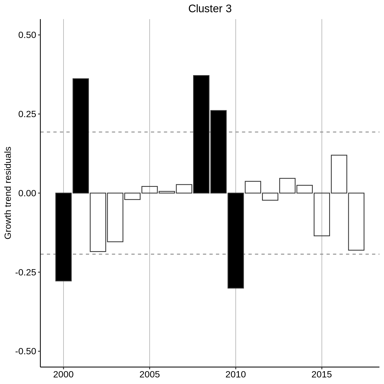
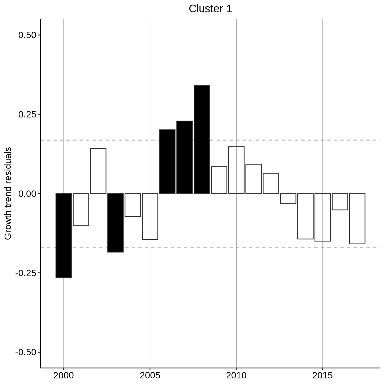
Recognizing an exponential growth, we perform a residual analysis by fitting an exponential curve to the general trend per cluster and evaluating the deviation from this general trend. We additionally flag if the residuals absolute values are greater than one-standard deviation of the residuals.
residual_year_cluster <- count_year_cluster %>%
  group_modify( ~ data.frame(
    year = .x$year,
    resid = lm(log(count + 1) ~ year, data = .x) %>% resid()
    ) %>%
  mutate(signif = resid > 0) %>%
  mutate(signif = ifelse(abs(resid) < sd(resid), NA, signif))
  )
residual_year_cluster
#> # A tibble: 54 x 4
#> # Groups:   cluster [3]
#>    cluster  year   resid signif
#>    <fct>   <dbl>   <dbl> <lgl>
#>  1 1        2000 -0.266  FALSE
#>  2 1        2001 -0.101  NA
#>  3 1        2002  0.143  NA
#>  4 1        2003 -0.184  FALSE
#>  5 1        2004 -0.0722 NA
#>  6 1        2005 -0.145  NA
#>  7 1        2006  0.201  TRUE
#>  8 1        2007  0.229  TRUE
#>  9 1        2008  0.341  TRUE
#> 10 1        2009  0.0850 NA
#> # … with 44 more rows
plot_fun <- function(.x, .title = .y$cluster){
  p <- ggplot(.x) +
    aes(x = year, y = resid, color = resid > 0, fill = signif) +
    theme_pubr(legend = "none") +
    scale_fill_manual(values = c("black","black")) +
    scale_color_manual(values = c("grey20","grey20")) +
    geom_hline(yintercept = sd(.x$resid), linetype="dashed", color="grey50") +
    geom_hline(yintercept = -sd(.x$resid), linetype="dashed", color="grey50") +
    labs(title = .title, y="Growth trend residuals") +
    theme(plot.title = element_text(hjust = 0.5)) +
    ylim(-.5, .5) +
    geom_bar(stat = "identity") +
    theme(axis.title.x = element_blank(), legend.position = "none") +
    scale_x_continuous(minor_breaks = seq(1980, 2020, by=1), breaks = seq(1980, 2020, 5)) +
    theme(panel.grid.major.x = element_line(size = .3, linetype = "solid", color = "grey62"))
    return(p)
}
residual_year_cluster %>% group_map(~  plot_fun(.x, .title = paste("Cluster", .y$cluster)))
#> [[1]]
#>
#> [[2]]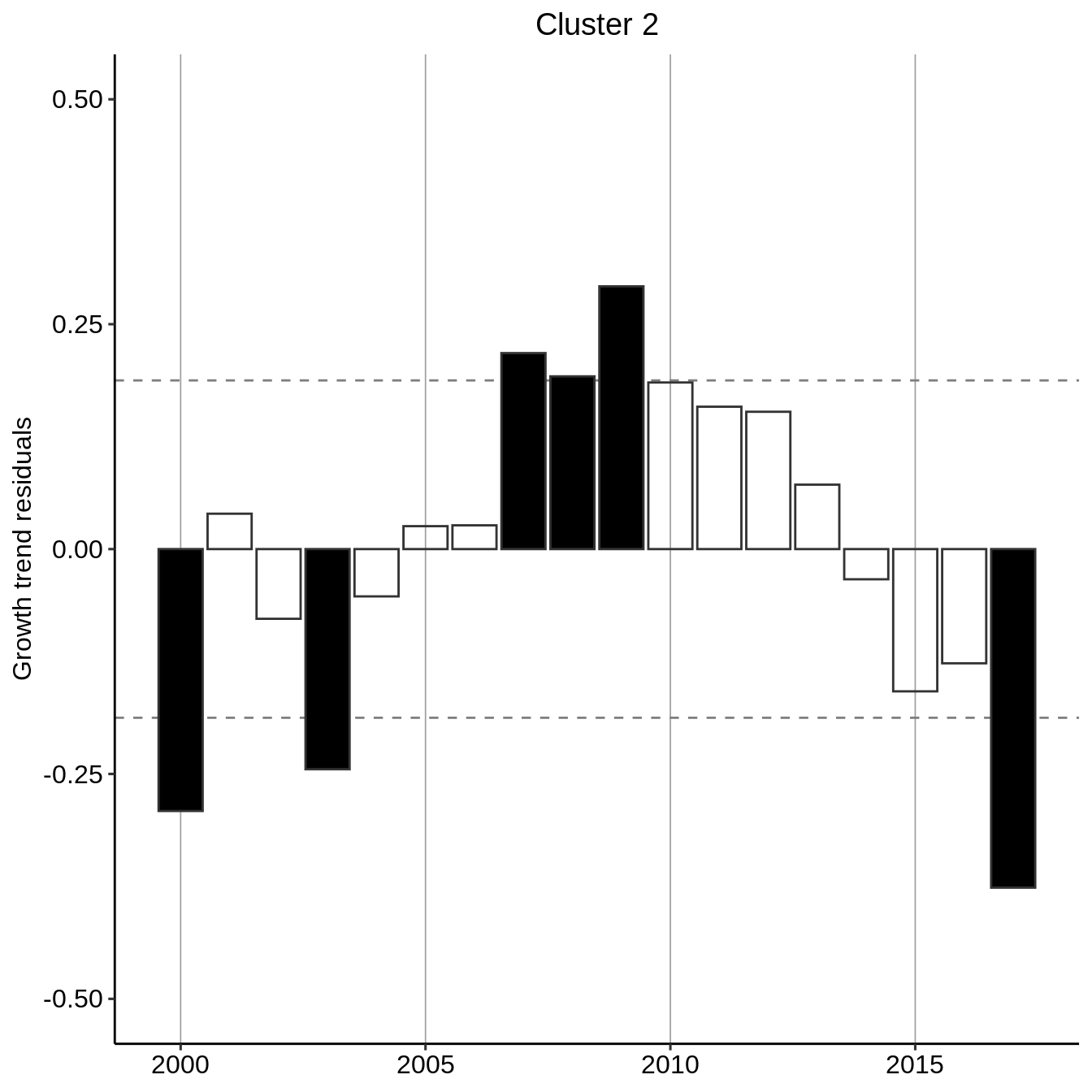
#>
#> [[3]]