Chord diagrams
chord_diagrams.RmdPurpose
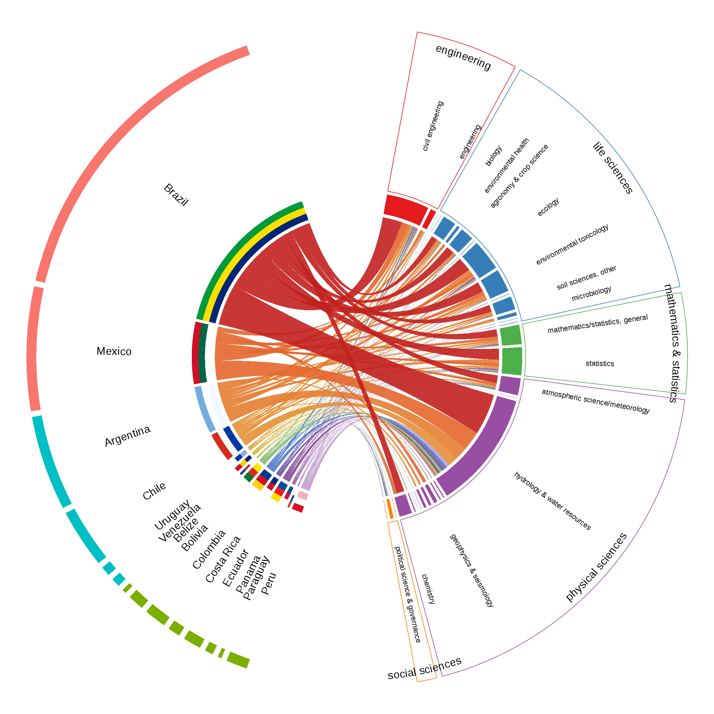
In this vignette, we produce a chord diagram representing the links of a weighted bi-partite network between countries and a category of topics.
Getting the bi-partite network weighted adjacency matrix
We use the built-in function of the package, get_network(), to extract the weighted adjacency matrix. We also load magrittr explicitely to access the %>% operator.
We select the specific topics with type = "NSF_specific", indicate that the country membership are to be understood as probabilities with prob = TRUE. The specific topics do not include methods, so we leave the default filter_method = FALSE which is useful for type = "theme". We display the default network with blindspot = FALSE, filter for countries with at least 30 documents with country.threshold = 30 and filter the resulting matrix to retain only the weights above the 75th percentile with percentile.threshold = .75.
weighted_adj_matrix <- get_network(type = "NSF_specific", prob = TRUE, filter_method = FALSE, blindspot = FALSE, country.threshold = 30, percentile.threshold = .75)
weighted_adj_matrix %>%
    knitr::kable(digits = 3, format = "html", caption = "Bi-partite network weighted adjacency matrix") %>%
    kableExtra::kable_styling(bootstrap_options = c("hover", "condensed")) %>%
    kableExtra::scroll_box(width = "7in")
| atmospheric science/meteorology | botany/plant biology | animal science | organic chemistry | biology | environmental health | mathematics/statistics, general | statistics | hydrology & water resources | civil engineering | oceanography, chemical and physical | agronomy & crop science | geomorphology | plant physiology | engineering | ecology | geophysics & seismology | environmental toxicology | geochemistry | sociology | ocean/marine science | environmental science | soil sciences, other | political science & governance | microbiology | analytical chemistry | marine biology & biological oceanography | geography | agricultural economics | forest science & biology | atmospheric chemistry & climatology | chemistry | |
|---|---|---|---|---|---|---|---|---|---|---|---|---|---|---|---|---|---|---|---|---|---|---|---|---|---|---|---|---|---|---|---|---|
| Venezuela | 8.250 | 0.000 | 0.000 | 4.969 | 0.000 | 0.000 | 4.767 | 5.640 | 27.797 | 7.771 | 0.000 | 0.000 | 0.000 | 4.943 | 0.000 | 7.422 | 0.000 | 7.138 | 5.084 | 0.000 | 0.000 | 0.00 | 0.000 | 0.000 | 0.000 | 0.000 | 0.000 | 0.000 | 0.000 | 0.00 | 0.000 | 5.443 |
| Uruguay | 0.000 | 0.000 | 5.262 | 0.000 | 6.638 | 0.000 | 5.816 | 9.549 | 28.692 | 7.958 | 0.000 | 4.867 | 0.000 | 0.000 | 0.000 | 11.874 | 0.000 | 4.392 | 0.000 | 0.000 | 4.166 | 0.00 | 0.000 | 0.000 | 7.578 | 0.000 | 0.000 | 0.000 | 0.000 | 0.00 | 0.000 | 0.000 |
| Peru | 0.000 | 0.000 | 0.000 | 0.000 | 0.000 | 0.000 | 11.272 | 11.868 | 78.623 | 18.395 | 16.120 | 0.000 | 11.564 | 0.000 | 15.894 | 9.523 | 0.000 | 0.000 | 0.000 | 0.000 | 11.421 | 0.00 | 0.000 | 18.824 | 0.000 | 0.000 | 0.000 | 0.000 | 0.000 | 0.00 | 10.807 | 0.000 |
| Paraguay | 1.648 | 0.000 | 0.000 | 0.000 | 1.444 | 0.000 | 2.052 | 3.158 | 15.016 | 3.196 | 1.423 | 0.000 | 1.610 | 0.000 | 0.000 | 3.926 | 0.000 | 1.610 | 0.000 | 0.000 | 0.000 | 0.00 | 0.000 | 2.549 | 0.000 | 0.000 | 0.000 | 0.000 | 0.000 | 0.00 | 0.000 | 0.000 |
| Panama | 6.634 | 3.756 | 0.000 | 0.000 | 0.000 | 0.000 | 4.676 | 6.943 | 25.342 | 5.393 | 4.019 | 0.000 | 0.000 | 3.996 | 0.000 | 9.493 | 0.000 | 0.000 | 0.000 | 0.000 | 0.000 | 0.00 | 4.144 | 0.000 | 0.000 | 0.000 | 0.000 | 0.000 | 0.000 | 9.82 | 0.000 | 0.000 |
| Mexico | 73.031 | 0.000 | 0.000 | 0.000 | 0.000 | 55.913 | 71.328 | 81.237 | 451.818 | 168.003 | 0.000 | 0.000 | 0.000 | 0.000 | 56.166 | 71.949 | 69.572 | 87.708 | 0.000 | 0.000 | 0.000 | 0.00 | 0.000 | 0.000 | 0.000 | 0.000 | 0.000 | 0.000 | 0.000 | 0.00 | 0.000 | 61.523 |
| Ecuador | 8.052 | 0.000 | 0.000 | 0.000 | 0.000 | 0.000 | 8.802 | 16.515 | 67.539 | 17.080 | 0.000 | 0.000 | 0.000 | 0.000 | 0.000 | 13.417 | 0.000 | 0.000 | 0.000 | 0.000 | 0.000 | 8.95 | 10.137 | 14.959 | 0.000 | 0.000 | 0.000 | 8.764 | 7.363 | 0.00 | 0.000 | 0.000 |
| Costa Rica | 7.648 | 0.000 | 0.000 | 0.000 | 0.000 | 0.000 | 7.114 | 7.066 | 49.035 | 9.390 | 0.000 | 6.250 | 0.000 | 0.000 | 0.000 | 14.747 | 5.605 | 6.311 | 0.000 | 0.000 | 0.000 | 0.00 | 5.950 | 0.000 | 0.000 | 5.683 | 0.000 | 0.000 | 0.000 | 0.00 | 0.000 | 0.000 |
| Colombia | 11.389 | 0.000 | 0.000 | 0.000 | 13.380 | 0.000 | 11.164 | 17.559 | 73.330 | 36.262 | 0.000 | 10.517 | 0.000 | 0.000 | 0.000 | 13.372 | 0.000 | 11.232 | 0.000 | 0.000 | 0.000 | 0.00 | 0.000 | 11.753 | 0.000 | 0.000 | 0.000 | 0.000 | 0.000 | 0.00 | 0.000 | 10.944 |
| Chile | 33.619 | 0.000 | 0.000 | 0.000 | 31.617 | 0.000 | 39.603 | 51.359 | 210.750 | 53.276 | 0.000 | 0.000 | 0.000 | 0.000 | 37.140 | 37.489 | 0.000 | 33.432 | 0.000 | 0.000 | 34.466 | 0.00 | 30.399 | 0.000 | 0.000 | 0.000 | 0.000 | 0.000 | 0.000 | 0.00 | 0.000 | 0.000 |
| Brazil | 181.605 | 0.000 | 0.000 | 0.000 | 145.425 | 0.000 | 168.396 | 257.991 | 963.390 | 452.171 | 0.000 | 186.354 | 0.000 | 0.000 | 0.000 | 327.887 | 0.000 | 241.606 | 0.000 | 0.000 | 0.000 | 0.00 | 161.130 | 0.000 | 0.000 | 0.000 | 0.000 | 0.000 | 0.000 | 0.00 | 0.000 | 178.712 |
| Bolivia | 9.610 | 0.000 | 0.000 | 0.000 | 0.000 | 0.000 | 8.304 | 8.430 | 59.439 | 16.431 | 0.000 | 7.006 | 8.176 | 0.000 | 9.130 | 0.000 | 0.000 | 0.000 | 0.000 | 7.953 | 0.000 | 0.00 | 0.000 | 18.223 | 0.000 | 0.000 | 0.000 | 0.000 | 0.000 | 0.00 | 9.493 | 0.000 |
| Belize | 2.194 | 0.000 | 0.000 | 0.000 | 3.511 | 0.000 | 0.000 | 2.699 | 11.701 | 3.083 | 0.000 | 0.000 | 3.857 | 0.000 | 0.000 | 3.823 | 0.000 | 2.005 | 0.000 | 0.000 | 0.000 | 0.00 | 1.993 | 0.000 | 0.000 | 0.000 | 3.752 | 0.000 | 0.000 | 0.00 | 2.691 | 0.000 |
| Argentina | 0.000 | 0.000 | 0.000 | 0.000 | 64.189 | 0.000 | 48.327 | 83.860 | 310.364 | 61.649 | 0.000 | 58.607 | 0.000 | 0.000 | 0.000 | 98.675 | 0.000 | 67.673 | 48.139 | 0.000 | 0.000 | 0.00 | 52.550 | 0.000 | 61.384 | 0.000 | 0.000 | 0.000 | 0.000 | 0.00 | 0.000 | 0.000 |
Chord diagram visualization
We can now use VizSpots() to display the chord diagram. This function is largely using the circlize library which documentation can be found here. weighted_adj_matrix is the matrix. We ask for the non-scaled results with scaled = FALSE, add the socio-hydrologic clusters colors with cluster_color = TRUE, and re-order the countries so that they are grouped by clusters with reorder_cluster = TRUE. We also add an outer ring identifying the general categories with NSF_general_color = TRUE. We have to specify here again the topic category with type = "NSF_specific". Finally, topic_threshold = .50 displays the topic which research volume in the corpus are above the 50th percentile.
VizSpots(weighted_adj_matrix, scaled = FALSE, cluster_color = TRUE, NSF_general_color = TRUE, type = "NSF_specific", topic_threshold = .50, reorder_cluster = TRUE)